Step-by-step tutorial

In this page, we show an up to date version the examples that are presented in the tutorial paper presented at DAIS 2021 (one of the three conferences of DisCoTec 2021).

This tutorial features some companion videos, embedded in this page.

Info

The tutorial is also available as a scientific document:

Info

All code has been open-sourced and it is being actively maintained on GitHub

Warning

Snapshots presented here are from the Java Swing GUI module that was the main UI at the time the tutorial was written, and may or may not reflect the current graphical appearance of the examples (which can be configured in any case).

Tip

Simulations in alchemist are written in YAML. YAML is pretty intuitive, it can be learnt quickly through Learn X in Y minutes Where X=yaml. Even without any prior knowledge, looking at the syntax and comparing it with the information in the aforementioned page should provide enough information.

Import the infrastructure

Warning

You need to be able to import an existing Gradle project from GitHub. If you have no idea of what I’m talking about, take a step back and make sure you followed the quickstart.

git clone https://github.com/DanySK/DisCoTec-2021-Tutorial.git
cd DisCoTec-2021-Tutorial
- Unix-like terminals: ./gradlew run00
- Windows terminals (cmd, Powershell): gradlew.bat run00

The shell should begin to work, download the required components, and pop a graphical interface in front of you.

Note

If something went wrong, let us know by opening an issue!

The build system is continuous-integration sensitive. If a GUI is not displayed but the proces terminates successfully, make sure that you do not have a CI environment variable set to true.

Writing and launching simple simulations

In this video you will see how to:

import the example project, and how to use it to run simulations;
write simple simulations in YAML;
deploy nodes into a bidimensional space; and
write programs that perform manipulation of data in form of tuples.

Note

This is actually the second video of the tutorial. The first presents introductory information on the simulator and its meta-model, it can be found in the Explanation chapter of the documentation.

The examples presented in the video are presented in the following subsections, updated to execute with the latest version of the simulator. You will find this code in the current version of the tutorial.

Tip

Make changes to the existing configuration files and see what happens!

Three connected devices

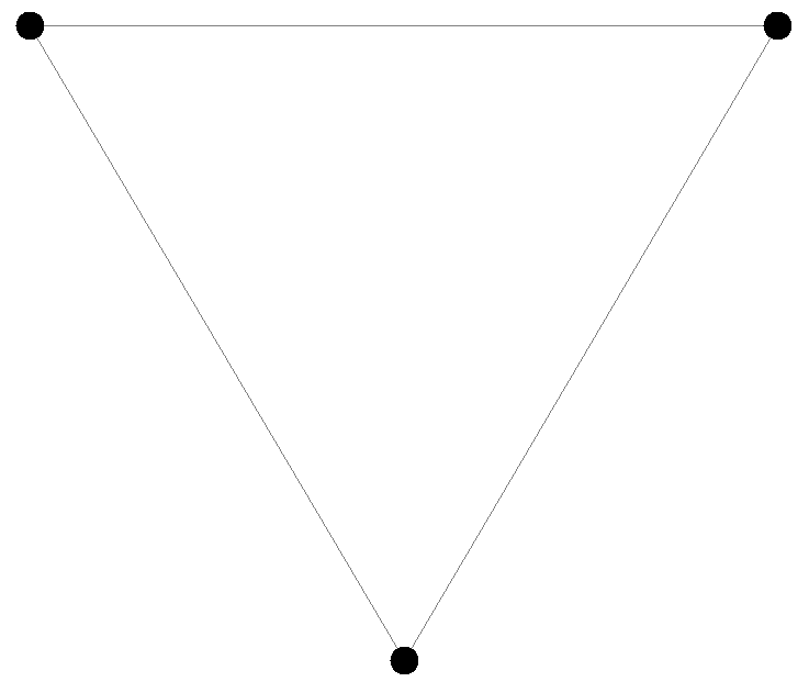
In this simple example, we simply deploy three nodes in a bidimensional space. They do nothing, they are just there. Starting the simulation would make it go to infinite time instantly, as there are no events to simulate.

Click to show / hide code

The graphic effect is just to see three dots in the interface. If links are displayed (see the reference of the graphical interface), then the three nodes appear linked.

Show snapshot

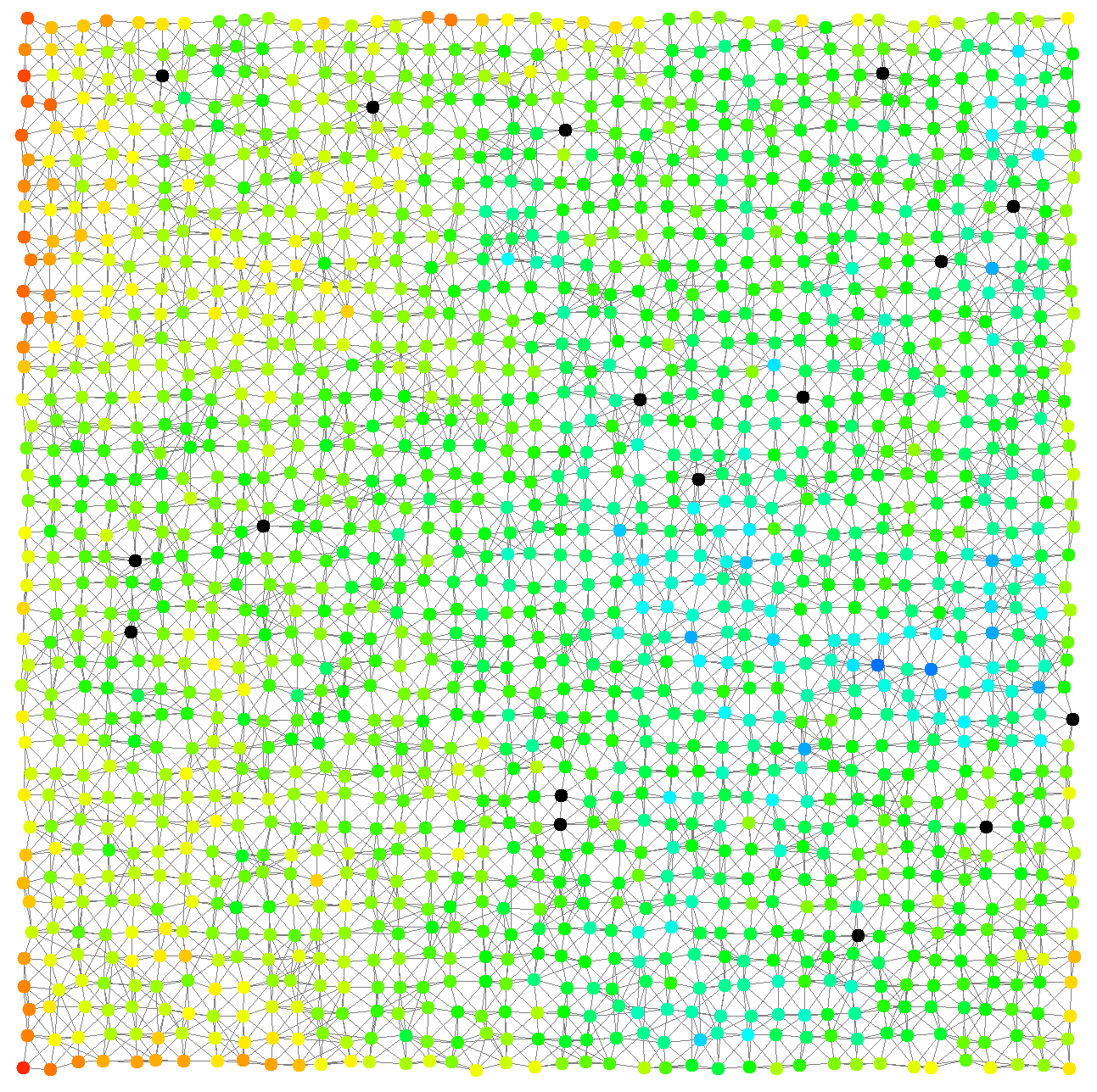
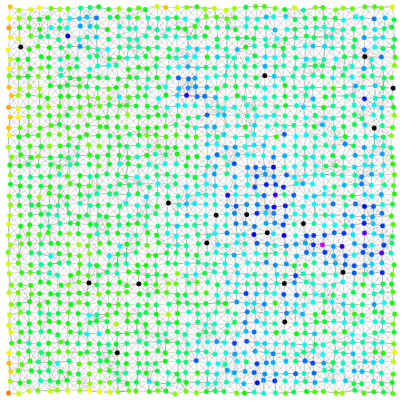
A grid of devices playing dodgeball

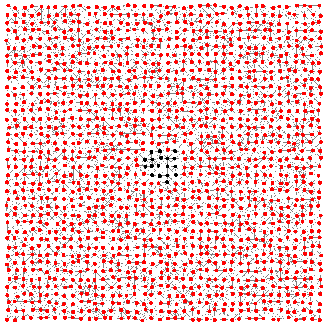
In this example we create a grid of devices and make them play dodgeball. The program to be injected is rather simple: some nodes will begin the simulation with a ball, and their goal will be to throw it to a random neighbor; whichever node gets hit takes a point, updates its score, and throws the ball again. This program is easy to write in a network of programmable tuple spaces, hence we write the following specification using the SAPERE incarnation.

Click to show / hide code

Snapshots of the simulation of the “dodgeball” example follow. Devices with a ball are depicted in black. All other devices’ color hue depends on the hit count, shifting from red (zero hits) towards blue.

Show snapshots

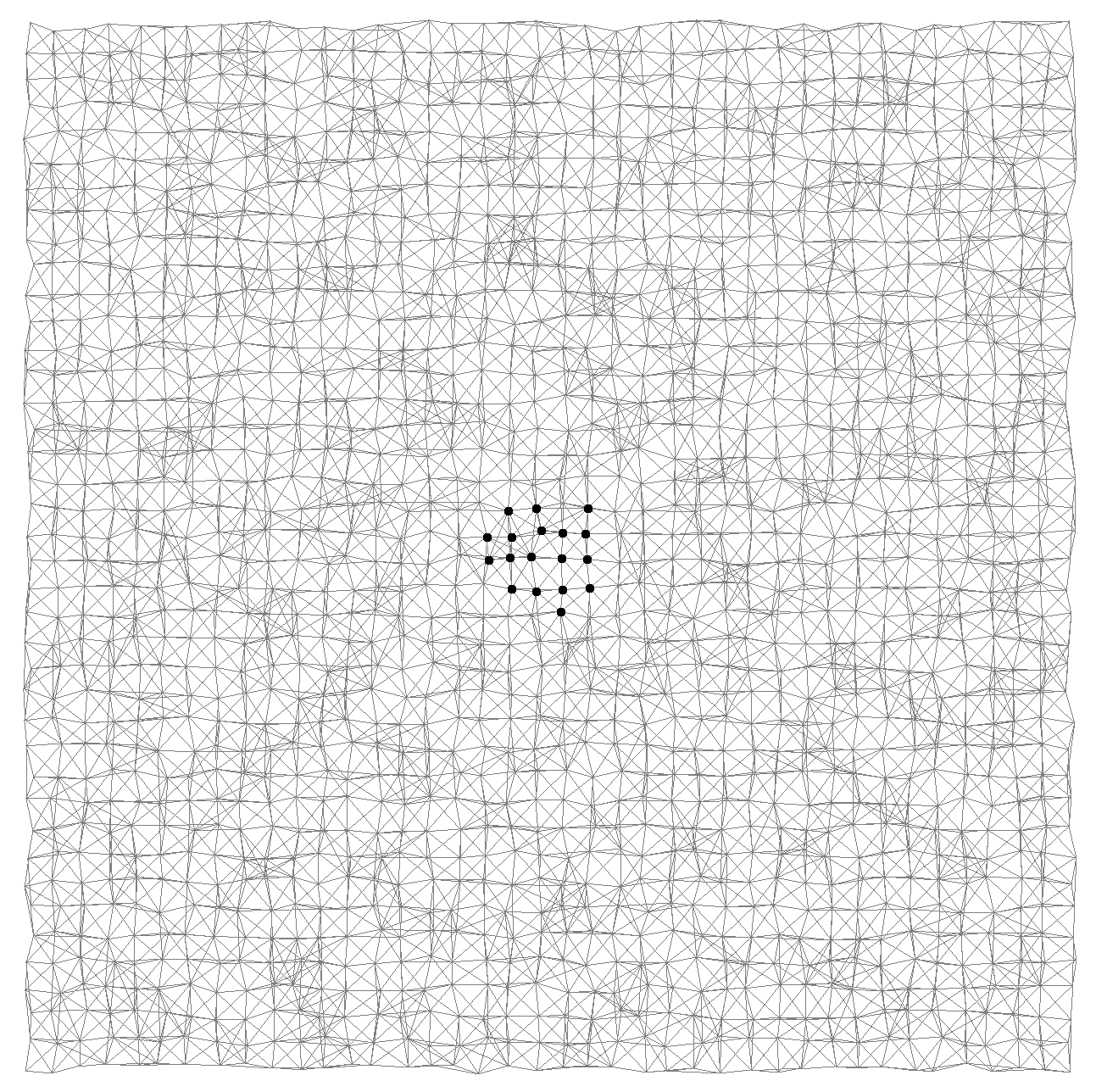
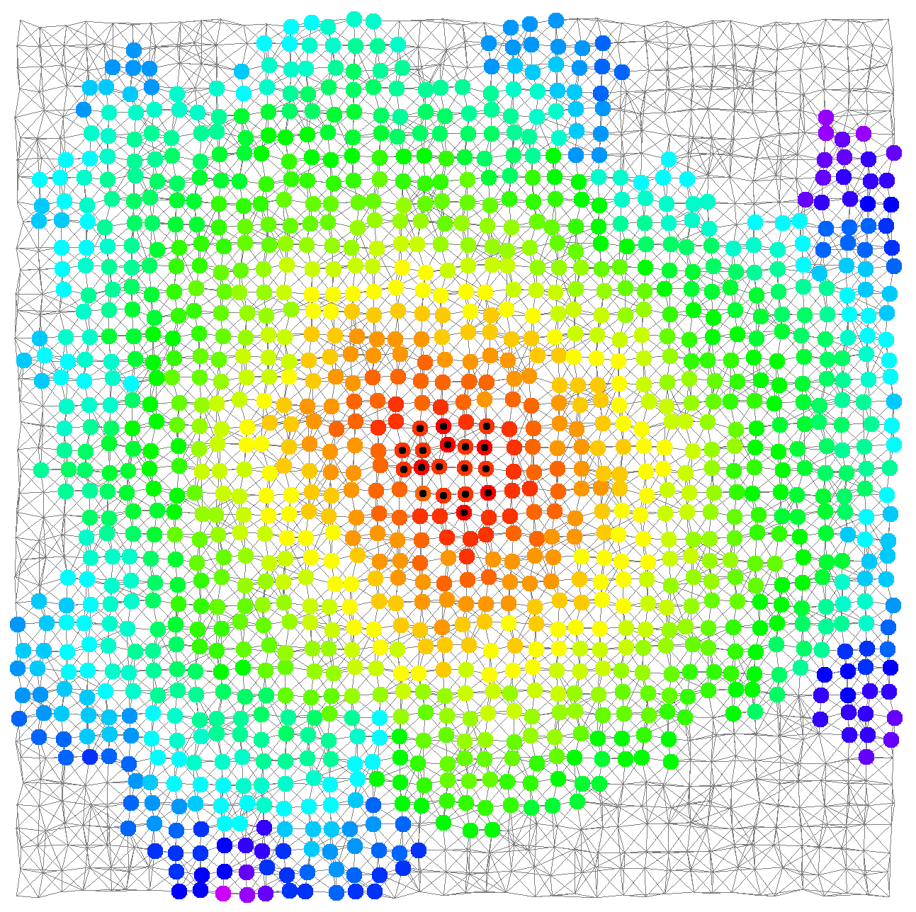
A gradient on a grid of devices

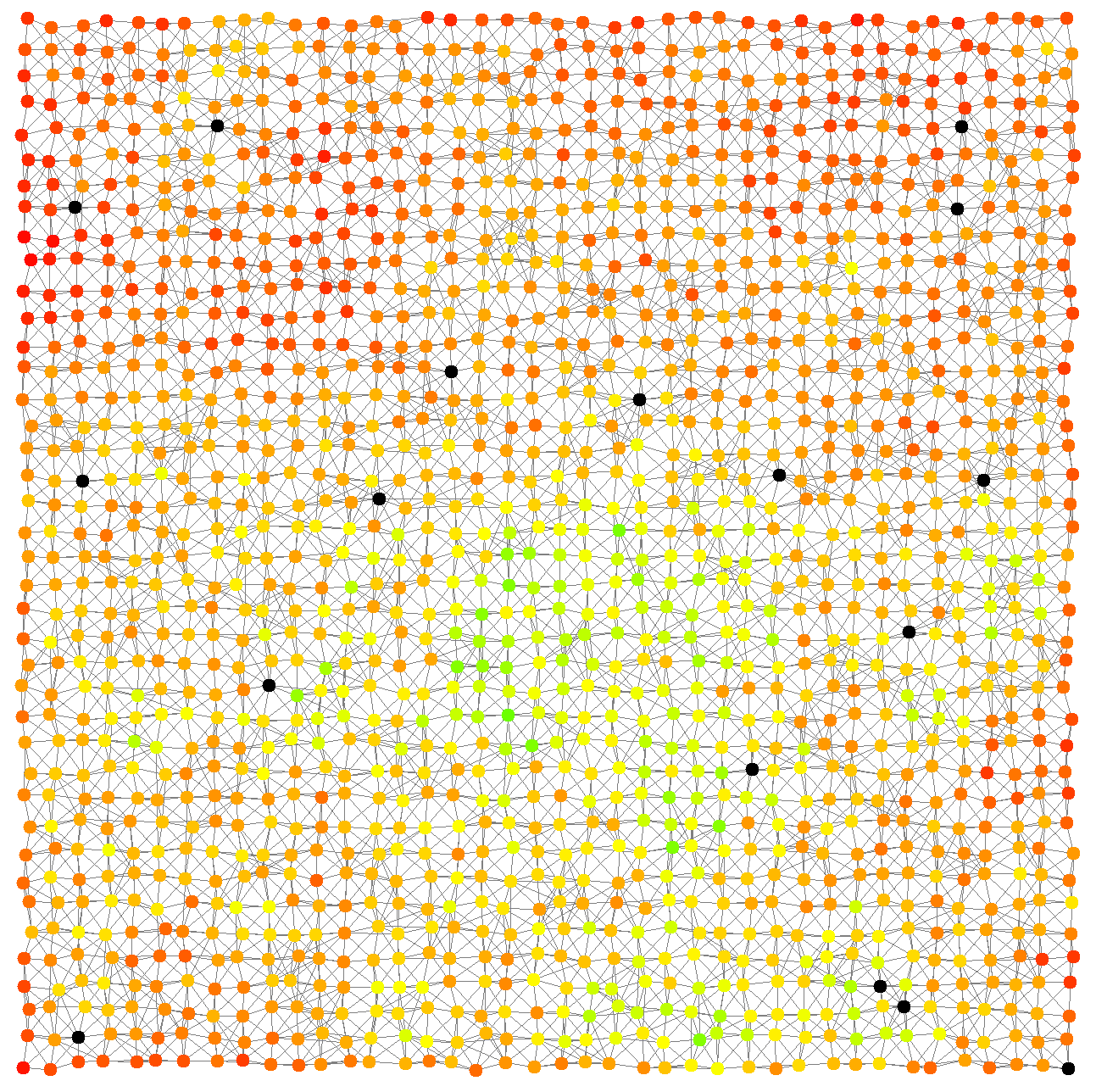
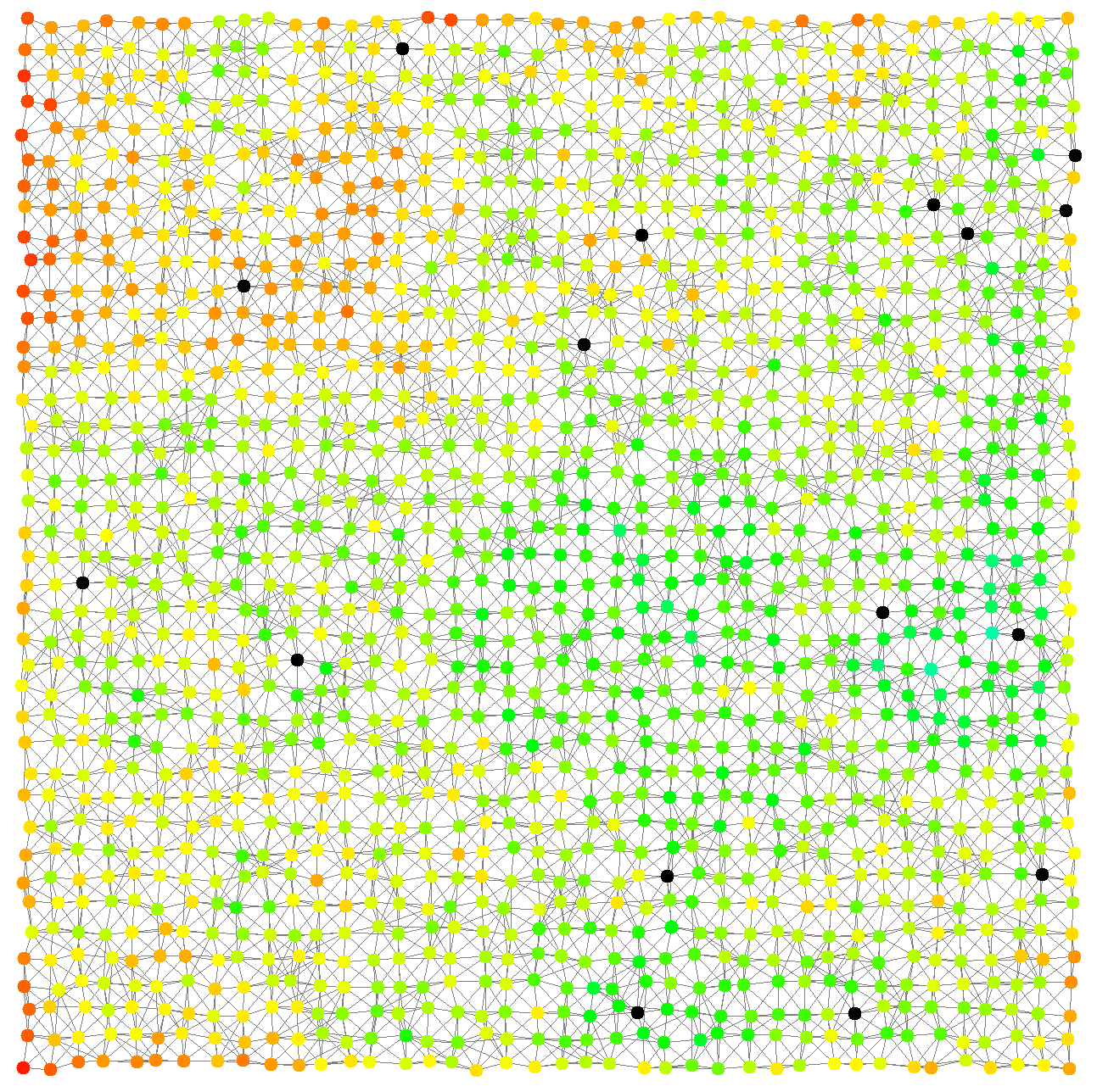
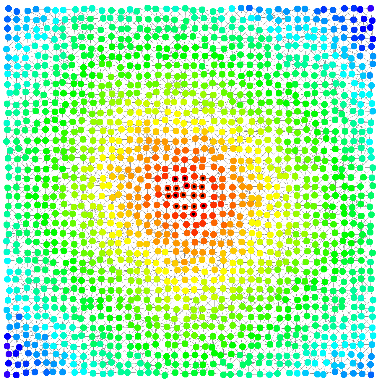
In this example, we implement with the SAPERE incarnation a very simple specification of a gradient, a pattern that is considered to be the basis of many other patterns ¹

Click to show / hide code

Here are some snapshots of the simulation of the “gradient” example. Source devices have a central black dot. Devices’ color hue depends on the gradient value, shifting from red (low) towards blue (high).

Show snapshots

Arbitrary network graphs

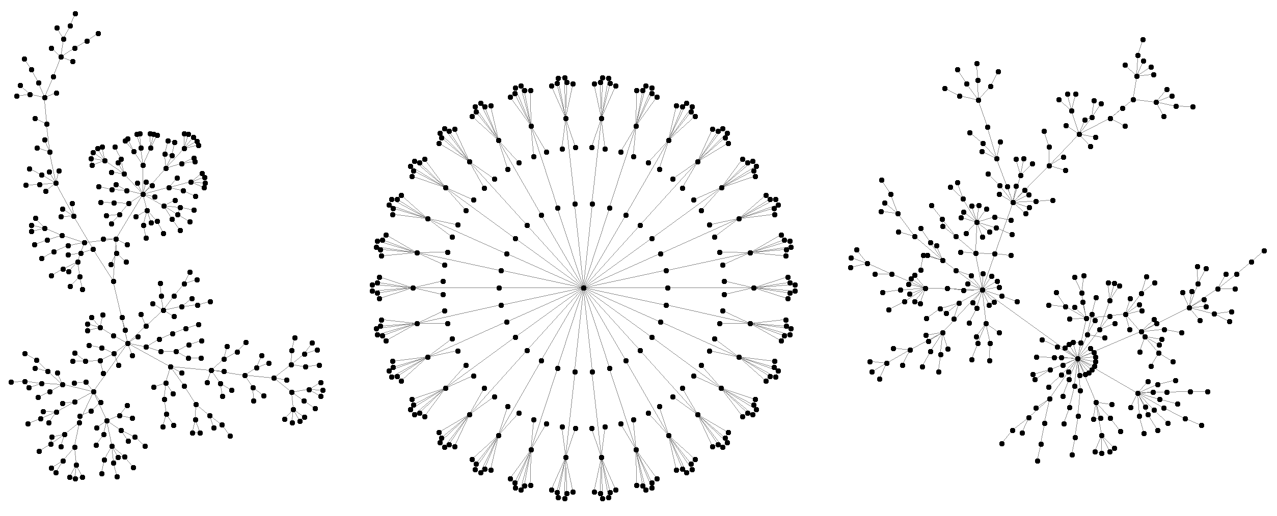
This example showcases some complex deployments made possible by Alchemist via Graphstream

Click to show / hide code

The example creates a single environment with three advanced deployments. From left to right: a Lobster graph, a banana tree, and a scale-free network with preferential attachment.

Advanced examples

In this video, we learn how to:

use aggregate programming (via Protelis) to write simulations;
use images to create indoor environments with physical obstacles;
use OpenStreetMap data to simulate on real-world maps; and
export data from simulations and configure batches exploring all possible combinations

Node mobility and indoor environments

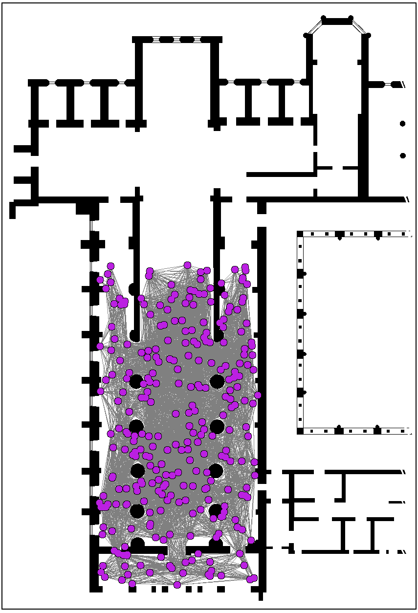
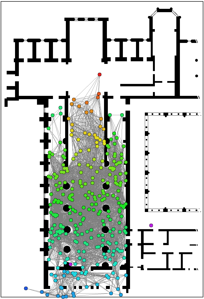
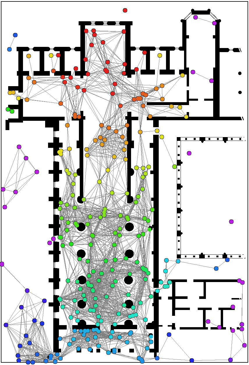
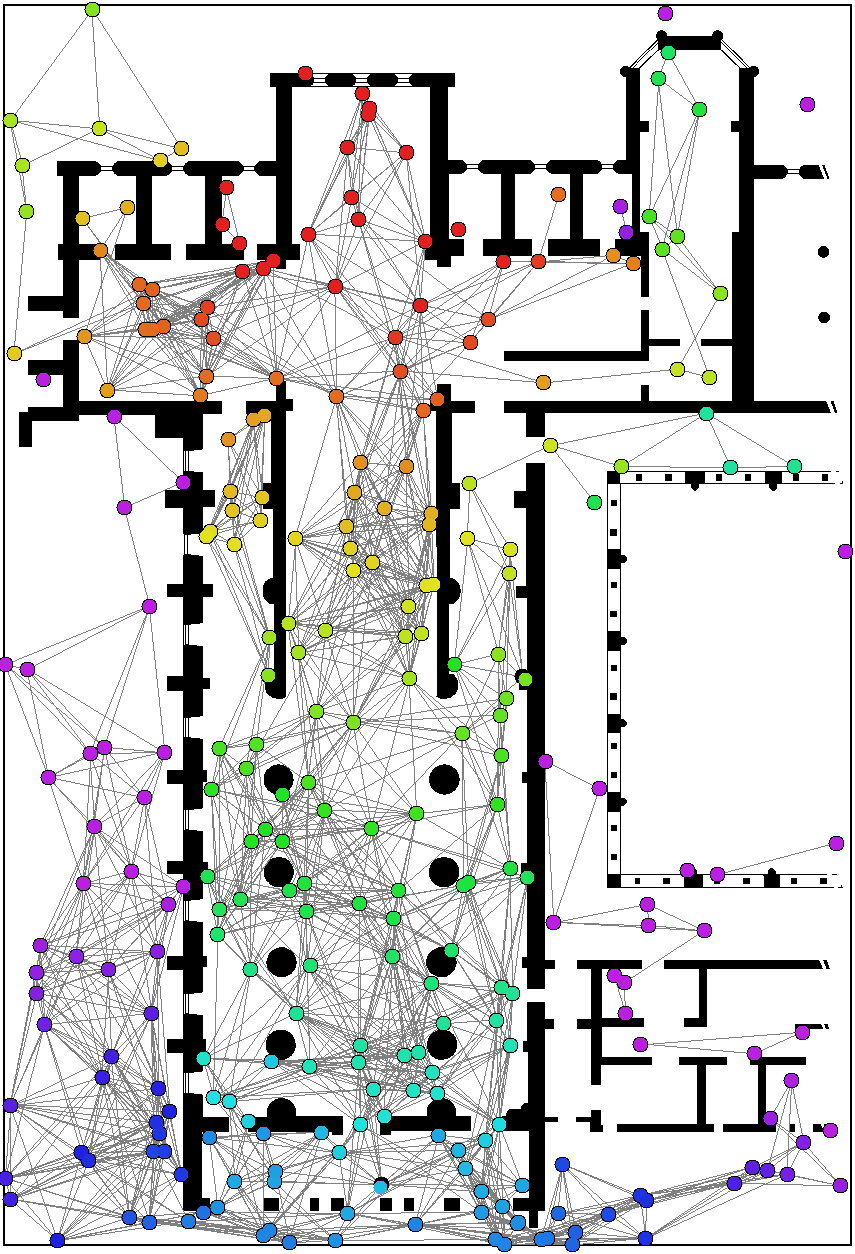
Many interesting scenarios the simulator targets require mobility and a richer environment. In the following example, we show a group of mobile devices estimating the distance from a point of interest (the altar) while moving within a church, whose planimetry has been taken from an existing building. Since the gradient is propagated in a network of mobile devices, we use a Protelis implementation of the adaptive Bellman-Ford algorithm from the Protelis-lang library²

Click to show / hide code

In the following snapshots, mobile devices progressively explore the location, while measuring the distance from a point of interest via gradient (red nodes are closer to the point of interest; purple ones are farther).

Show snapshots

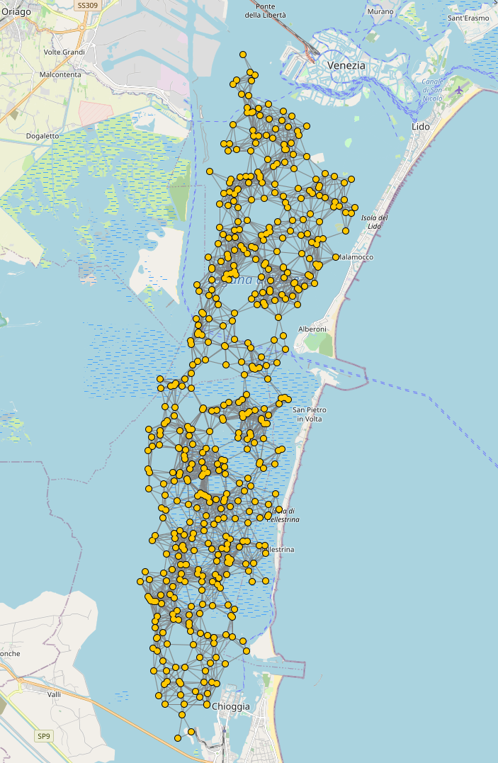
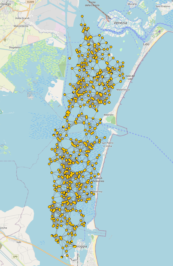
Real-world maps and GPS traces

The simulator can load data from OpenStreetMap exports, navigate devices towards a destination along streets by relying on GraphHopper or by using GPS traces in GPX format, or even using the navigation system to interpolate sparse GPS traces, thus preventing nodes from taking impossible paths. In the following simple scenario buoys are deployed in the Venice lagoon and move Brownianly.

Click to show / hide code

The following snapshots depict the simulation in execution.

Show snapshots

In-depth analysis of simulated scenarios

The following snippet showcases the aforementioned features by enriching the example of a gradient in an indoor environment presented previously with:

variables for the pedestrian walking speed, pedestrian count, and random seed;
constants to ease the configuration of the simulation;
a Kotlin resource search expressed as a variable;
controlled reproducibility by controlling random seeds;
export of generated data (time and several statistics on the gradient).

Click to show / hide code

incarnation: protelis
variables:
  zoom: &zoom
    formula: 0.1 # Must be a valid Groovy snippet
  image_name: { formula: "'chiaravalle.png'" }
  image_path: &image_path
    language: kotlin # Pick whatever JSR223 language you like and add it to the classpath
    formula: | # The following is pure Kotlin code. Other variables can be referenced!
      import java.io.File
      fun File.findImage(): String? = walkTopDown().find { image_name in it.name }?.absolutePath
      fun File.findImageRecursively(): String = findImage() ?: File(this, "..").findImageRecursively()
      File(".").findImageRecursively()
    timeout: 5000
  # Linear free variable
  walking_speed: &walk-speed { default: 1.4, min: 1, max: 2, step: 0.1 }
  seed: &seed { default: 0, min: 0, max: 99, step: 1 } # 100 samples
  scenario_seed: &scenario_seed { formula: (seed + 31) * seed } # Variable-dependent
  people_count: &people_count
    type: GeometricVariable # A variable scanning a space with geometric segmentation
    parameters: [300, 50, 500, 9] # default 300, minimum 50, maximum 100, 9 samples
seeds: { simulation: *seed, scenario: *scenario_seed}
export:
    type: CSVExporter
    parameters:
      fileNameRoot: "snippet-variables-export"
    data:
      - time
      - molecule: "default_module:default_program"
        aggregators: [ mean, max, min, variance, median ] # From Apache's UnivariateStatistic
        value-filter: onlyfinite # discards NaN and Infinity
environment: { type: ImageEnvironment, parameters: [*image_path, *zoom] }
network-model: { type: ObstaclesBreakConnection, parameters: [50] }
deployments:
  type: Rectangle
  parameters: [*people_count, 62, 15, 95, 200]
  programs:
    - time-distribution: 1
      program: >
        import protelis:coord:spreading
        let source = [110, 325]
        let vector = self.getCoordinates() - source
        let distance = hypot(vector.get(0), vector.get(1))
        distanceTo(distance < 50)        
    - program: send
    - { type: Event, time-distribution: 1, actions: { type: LevyWalk, parameters: [*walk-speed] } }

Info

This example:

↩︎
↩︎