Coordination 2021 (one of the three conferences of DisCoTec 2021) is about to host an Alchemist tutorial. In this page, we show an up to date version the examples that are presented in the tutorial paper. Snapshots are from the Java Swing GUI module that was the main UI at the time the tutorial was written, and may or may not reflect the current graphical appearance of the examples (which can be configured in any case). Further details on the examples are available in the tutorial paper.

Three connected devices

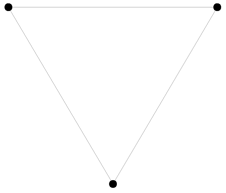
In this simple example, we simply deploy three nodes in a bidimensional space.

incarnation: sapere # The incarnation is always mandatory
network-model:
  type: ConnectWithinDistance # Loads a class with this name implementing LinkingRule
  parameters: [2] # Connection radius (parameter of a ConnectWithinDistance's constructor)
deployments:
  - type: Point # Loads a class with this name implementing Deployment
    parameters: [0, 0] # Coordinates
  - { type: Point, parameters: [0.5, 0.85] }
  - { type: Point, parameters: [-0.5, 0.85] }

A grid of devices playing dodgeball

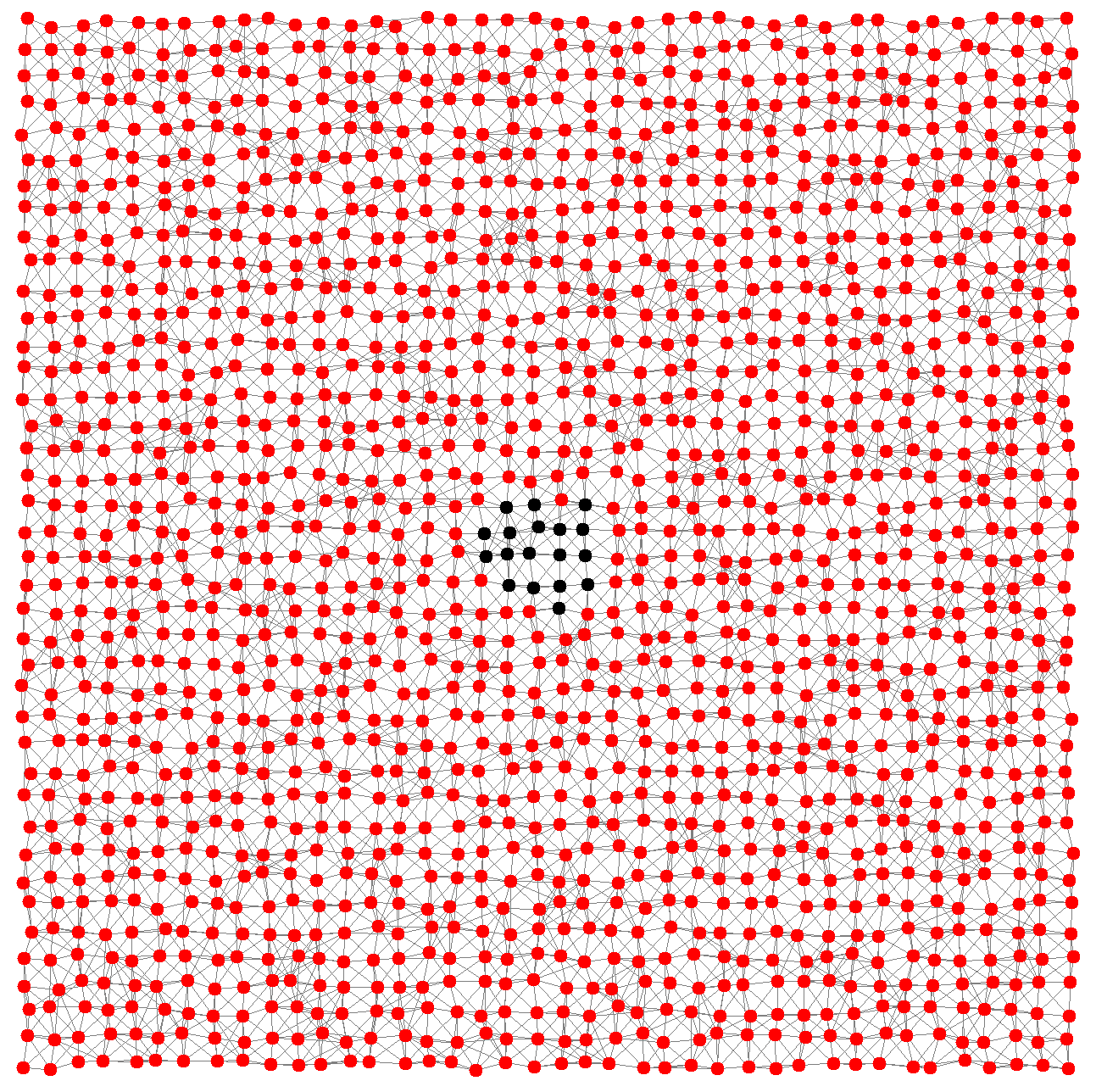
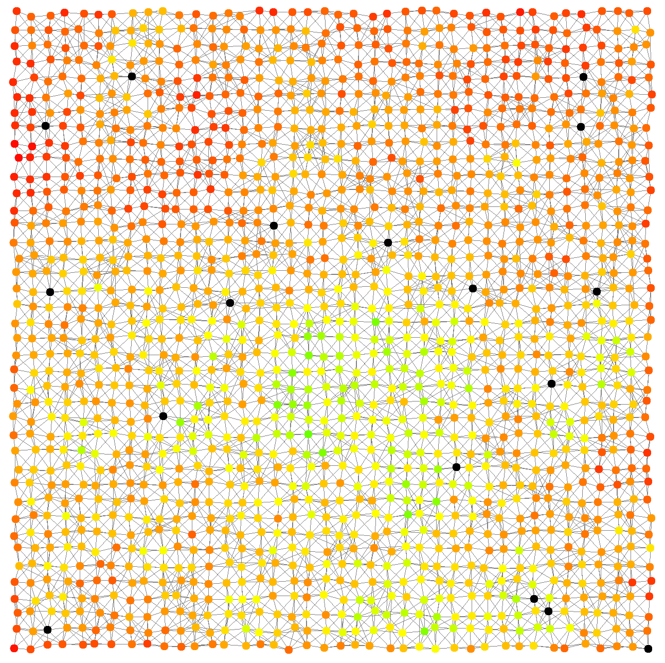
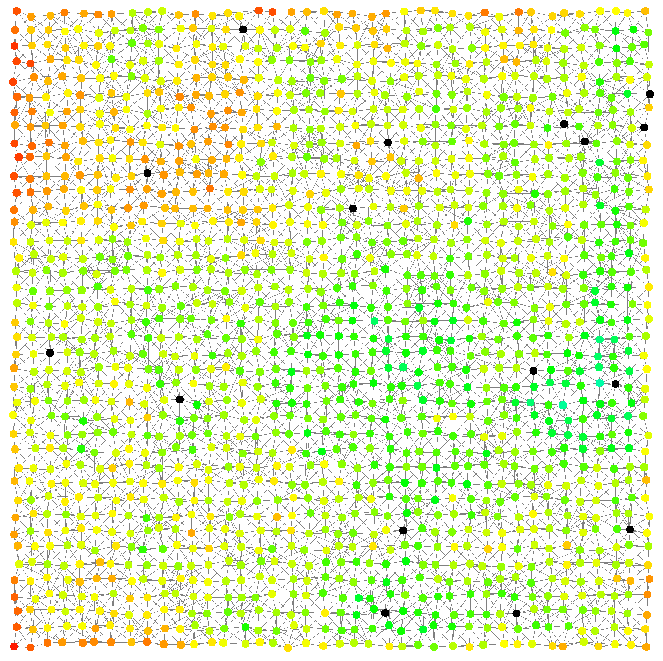
In this example we create a grid of devices and make them play dodgeball. The program to be injected is rather simple: some nodes node will begin the simulation with a ball, and their goal will be to throw it to a random neighbor; whichever node gets hit takes a point, updates its score, and throws the ball again. This program is easy to write in a network of programmable tuple spaces, hence we write the following specification using the SAPERE incarnation.

incarnation: sapere
network-model: { type: ConnectWithinDistance, parameters: [0.5] }
deployments:
  type: Grid
  parameters: [-5, -5, 5, 5, 0.25, 0.25, 0.1, 0.1] # A perturbed grid of devices
  contents:
    - molecule: "{hit, 0}" # Everywhere, no one has been hit
    - in: { type: Rectangle, parameters: [-0.5, -0.5, 1, 1] } # Inside this shape...
      molecule: ball # ...every node has a ball
  programs:
    - time-distribution: 1 # This is a frequency, time distribution type is left to the incarnation
      # 'program' specs are passed down to the incarnation for being interpreted as reactions
      program: "{ball} {hit, N} --> {hit, N + 1} {launching}" # If hit, count the hit
    - program: "{launching} --> +{ball}" # As soon as possible, throw the ball to a neighbor

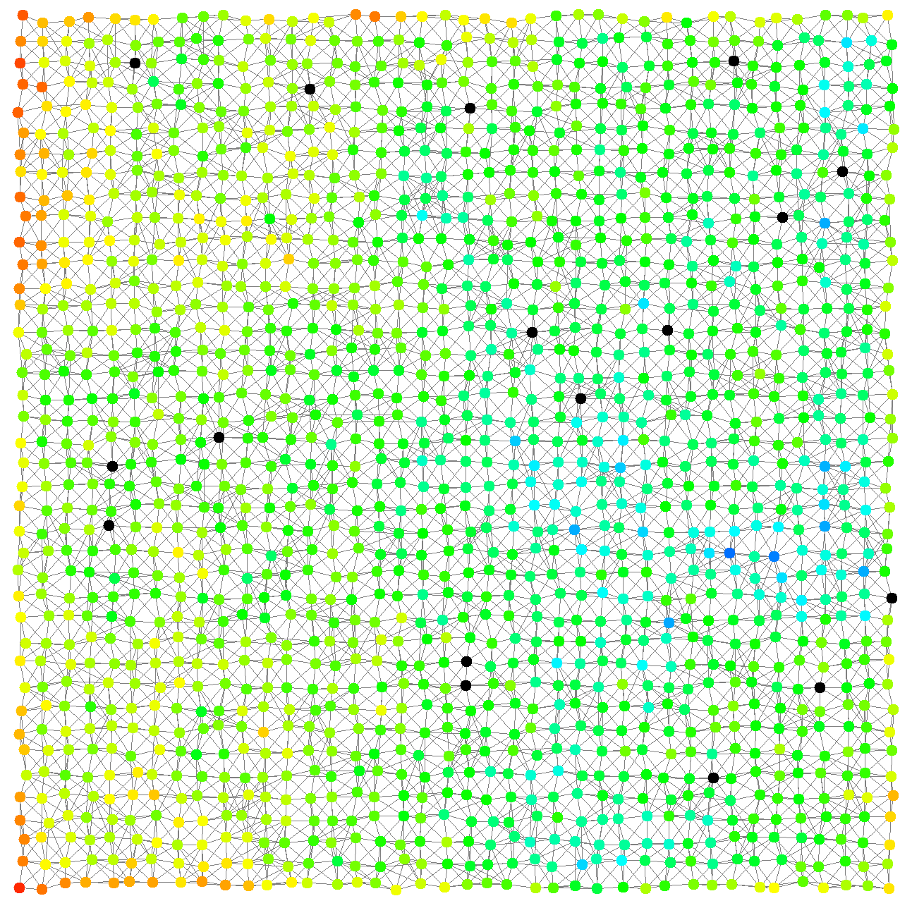
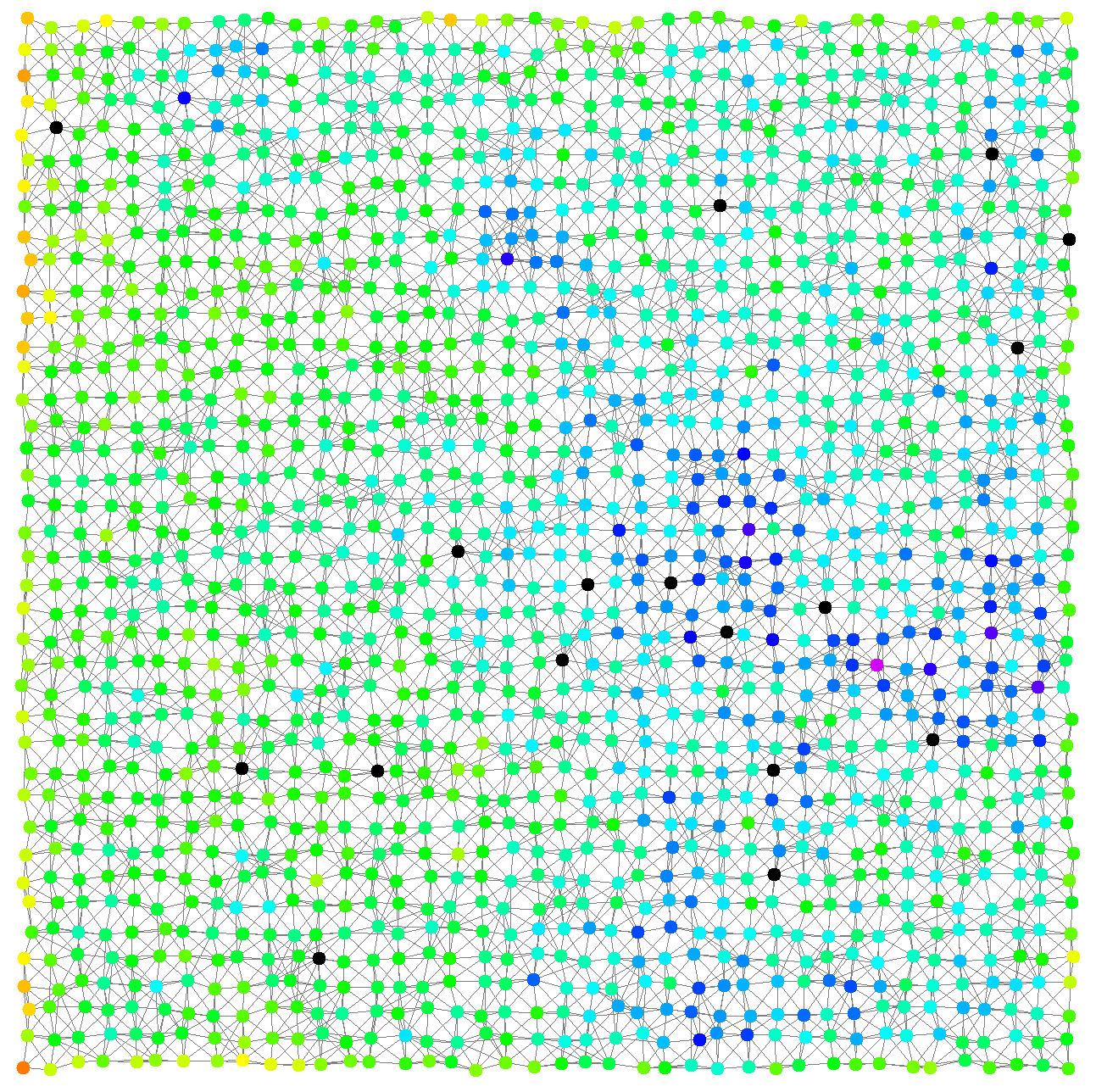
Snapshots of the simulation of the “dodgeball” example follow. Devices with a ball are depicted in black. All other devices’ color hue depends on the hit count, shifting from red (zero hits) towards blue.

A gradient on a grid of devices

In this example, we implement with the SAPERE incarnation a very simple specification of a gradient, a pattern that is considered to be the basis of many other patterns.

incarnation: sapere
network-model: { type: ConnectWithinDistance, parameters: [0.5] }
deployments:
  type: Grid
  parameters: [-5, -5, 5, 5, 0.25, 0.25, 0.1, 0.1]
  contents:
    in: { type: Rectangle, parameters: [-0.5, -0.5, 1, 1] }
    molecule: source # Here is the source of the gradient
  programs:
    - time-distribution: 0.1 # Exponential with λ=0.1
      # If there is a source, then the gradient is zero.
      program: "{source} --> {source} {gradient, 0}"
    - time-distribution: 1 # Exponential distribution with λ=1
      # Send all neighbors your gradient value plus one
      program: "{gradient, N} --> {gradient, N} *{gradient, N+1}"
      # In case of multiple gradients, take the shortest
    - program: "{gradient, N}{gradient, def: N2>=N} --> {gradient, N}"
    - time-distribution: 0.1
      program: "{gradient, N} --> {gradient, N + 1}" # Aging process
    - program: "{gradient, def: N > 30} -->" # Death process

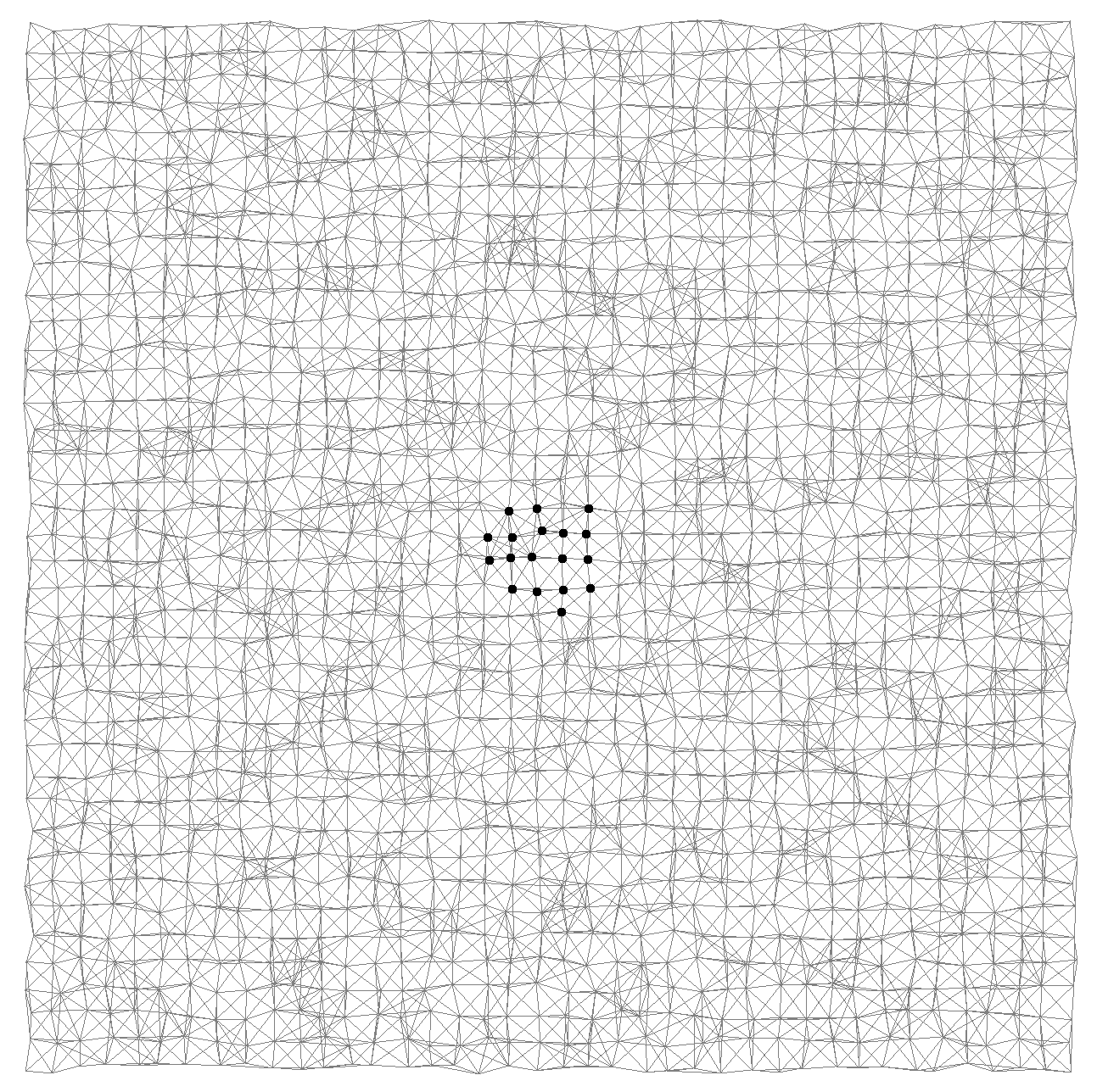
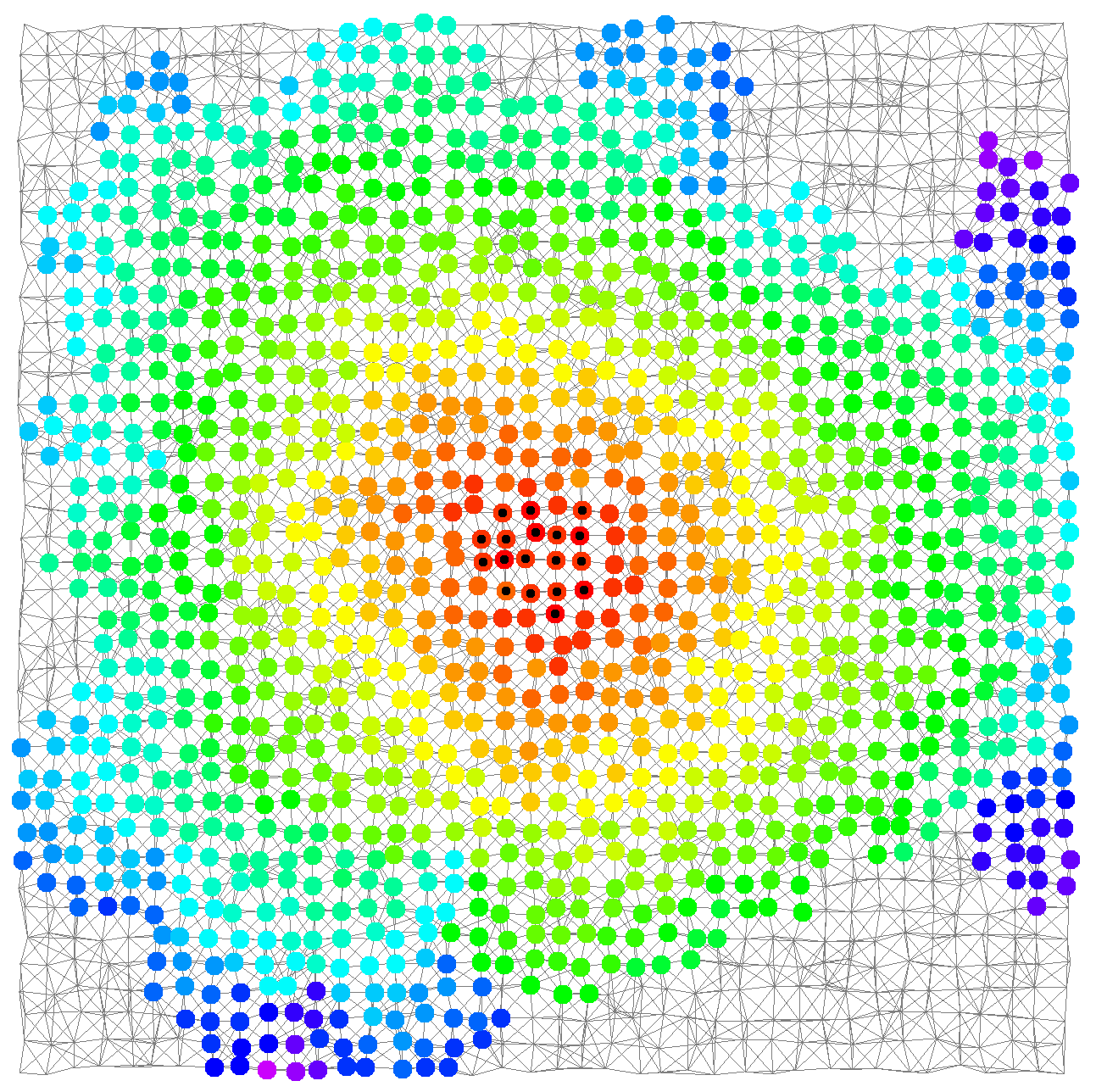
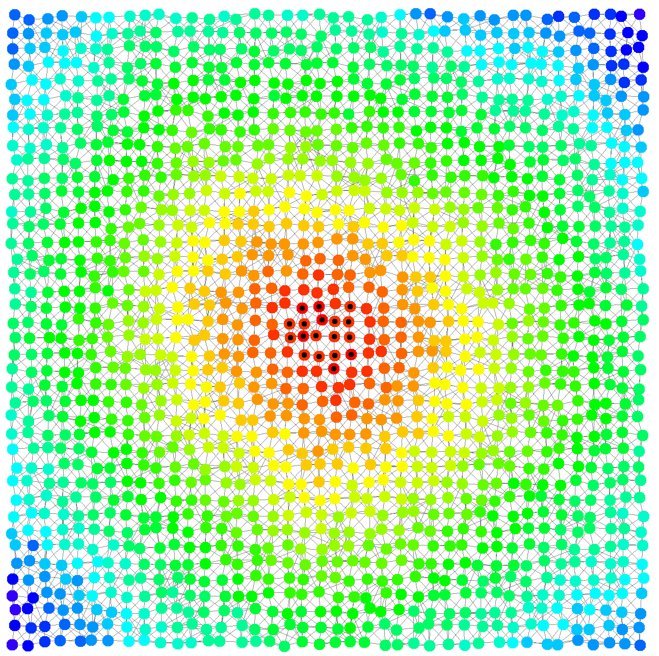
Here are some snapshots of the simulation of the “gradient” example. Source devices have a central black dot. Devices’ color hue depends on the gradient value, shifting from red (low) towards blue (high).

Arbitrary network graphs

This example showcases some complex deployments made possible by Alchemist via Graphstream

incarnation: sapere
network-model: { type: ConnectWithinDistance, parameters: [0.5] }
deployments:
  - { type: GraphStreamDeployment, parameters: [300, -30, 0, 0.8, Lobster, [5, 15]] }
  - { type: GraphStreamDeployment, parameters: [300, 0, 0, 2, BananaTree, 10] }
  - { type: GraphStreamDeployment, parameters: [300, 30, 0, PreferentialAttachment] }

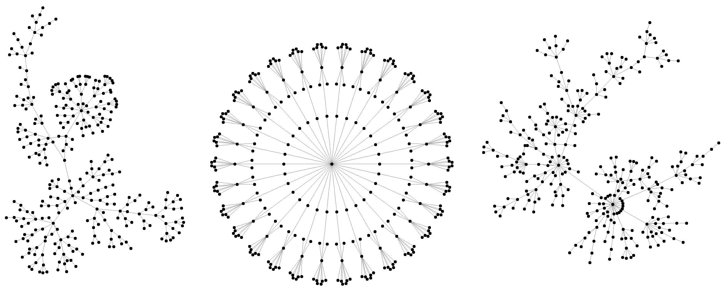
The example creates a single environment with three advanced deployments. From left to right: a Lobster graph, a banana tree, and a scale-free network with preferential attachment.

Node mobility and indoor environments

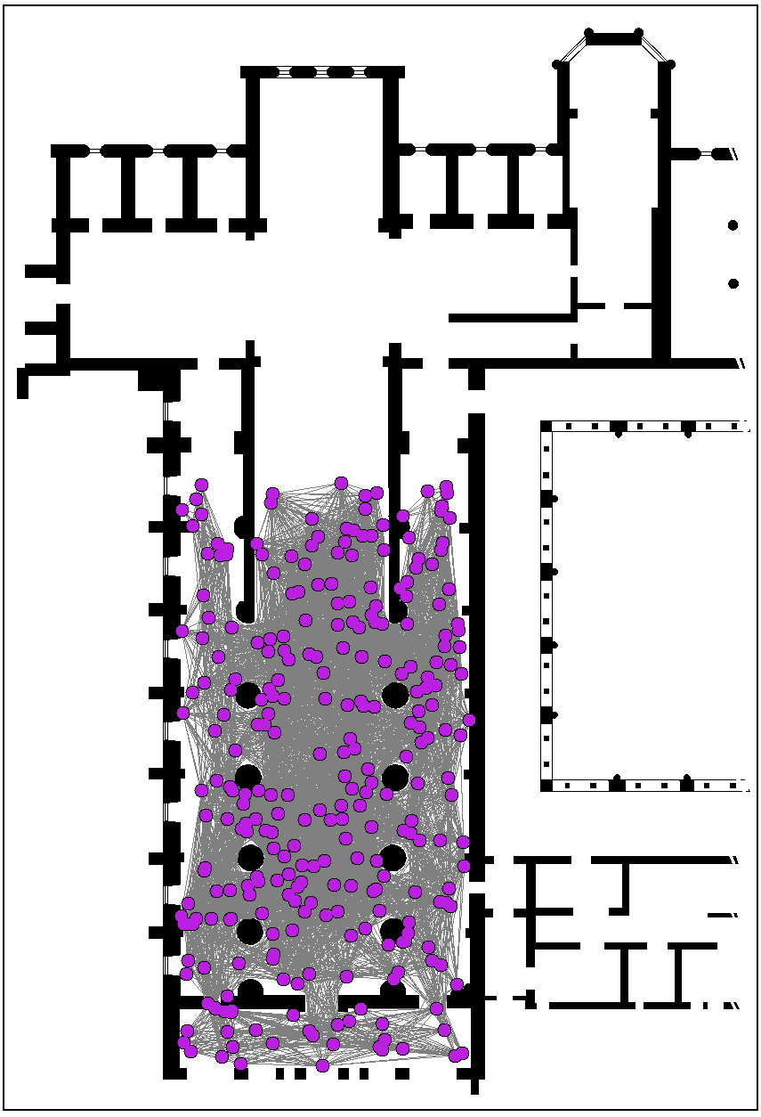
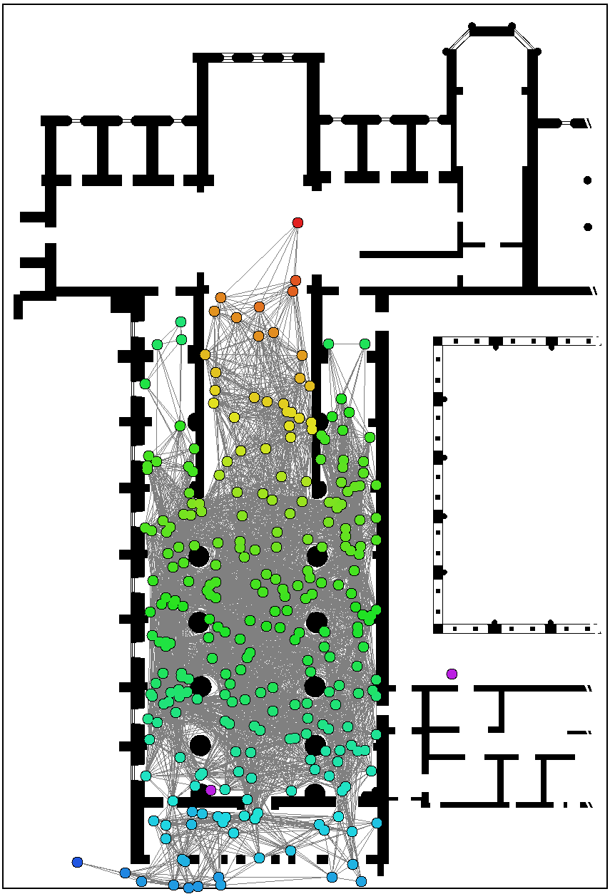
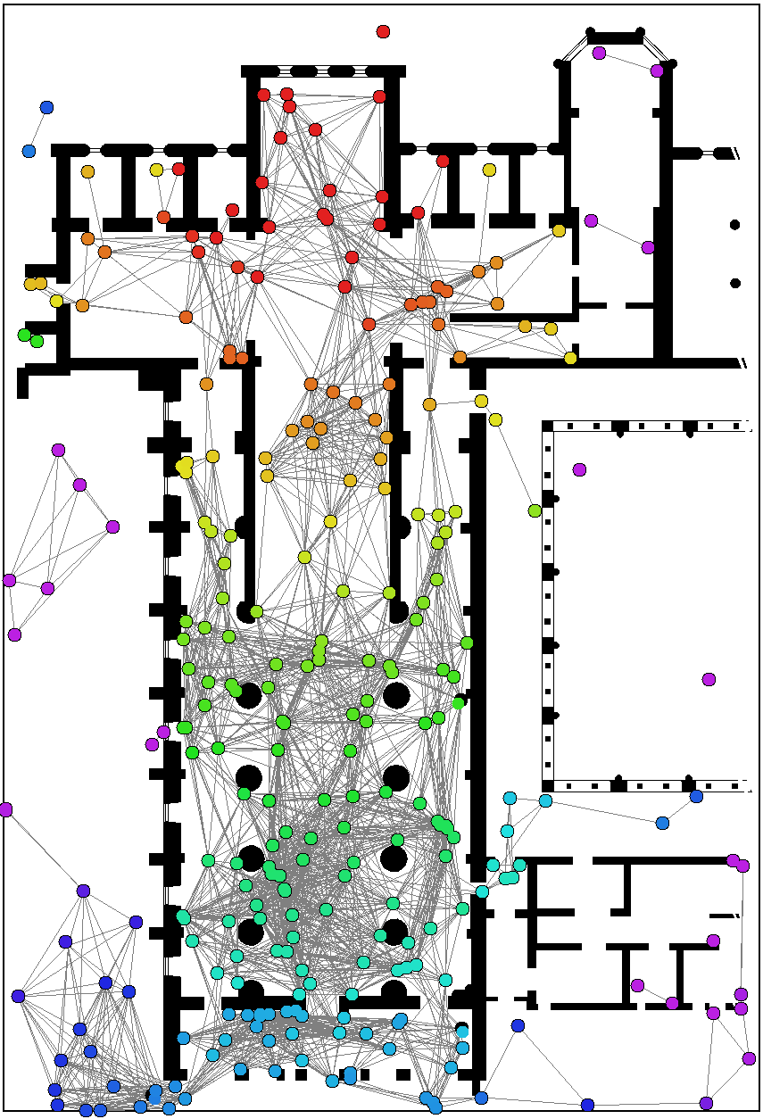
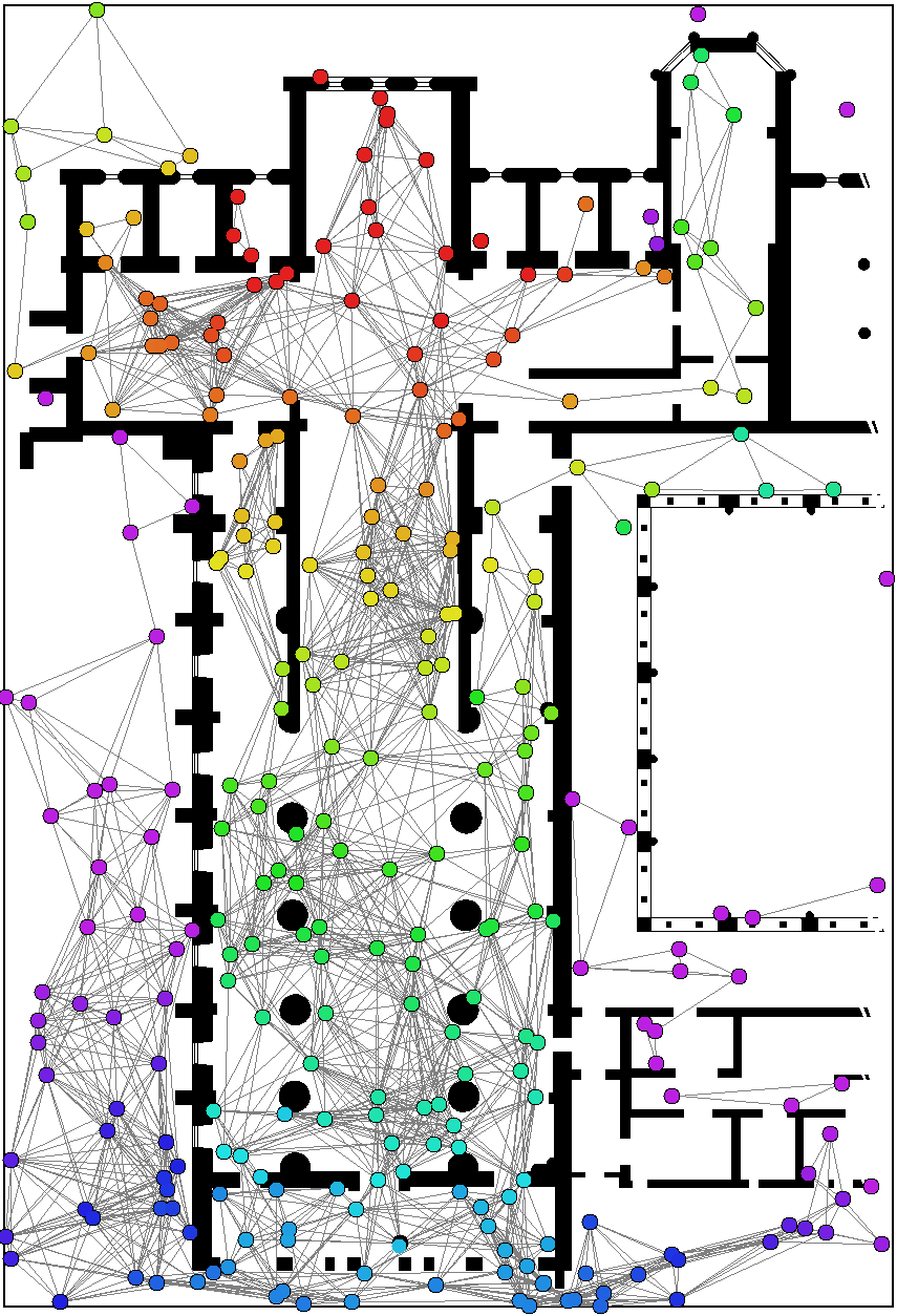
many interesting scenarios the simulator targets require mobility and a richer environment. In the following example, we show a group of mobile devices estimating the distance from a point of interest (the altar) while moving within a church, whose planimetry has been taken from an existing building. Since the gradient is propagated in a network of mobile devices, we use a Protelis implementation of the adaptive Bellman-Ford algorithm from the Protelis-lang library.

incarnation: protelis
environment: { type: ImageEnvironment, parameters: [chiaravalle.png, 0.1] }
network-model: { type: ObstaclesBreakConnection, parameters: [50] }
deployments:
  type: Rectangle
  parameters: [300, 62, 15, 95, 200]
  programs:
    - time-distribution: 1
      program: >
        import protelis:coord:spreading
        let source = [110, 325]
        let vector = self.getCoordinates() - source
        let distance = hypot(vector.get(0), vector.get(1))
        distanceTo(distance < 50)
    - program: send # Actual network message delivery
    - type: Event
      time-distribution: 1
      actions: { type: LevyWalk, parameters: [1.4] }

In the following snapshots, mobile devices progressively explore the location, while measuring the distance from a point of interest via gradient (red nodes are closer to the point of interest; purple ones are farther).

Real-world maps and GPS traces

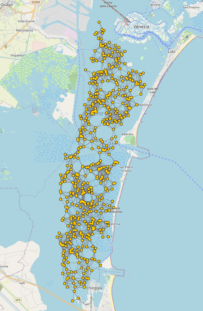
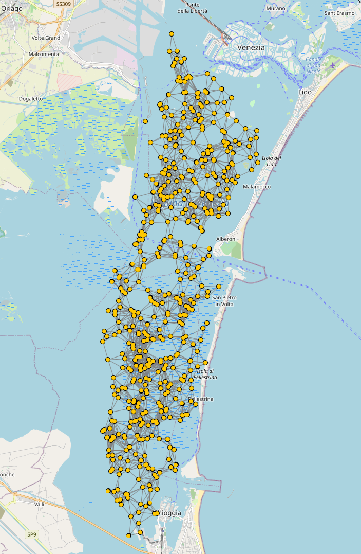
The simulator can load data from OpenStreetMap exports, navigate devices towards a destination along streets by relying on GraphHopper8 or by using GPS traces in GPX format, or even using the navigation system to interpolate sparse GPS traces, thus preventing nodes from taking impossible paths. In the following simple scenario buoys are deployed in the Venice lagoon and move Brownianly.

incarnation: sapere
environment: { type: OSMEnvironment }
network-model: { type: ConnectWithinDistance, parameters: [1000] }
_venice_lagoon: &lagoon
  [[45.2038121, 12.2504425], [45.2207426, 12.2641754], [45.2381516, 12.2806549],
   [45.2570053, 12.2895813], [45.276336, 12.2957611], [45.3029049, 12.2991943],
   [45.3212544, 12.3046875], [45.331875, 12.3040009], [45.3453893, 12.3040009],
   [45.3502151, 12.3156738], [45.3622776, 12.3232269], [45.3719259, 12.3300934],
   [45.3830193, 12.3348999], [45.395557, 12.3445129], [45.3998964, 12.3300934],
   [45.4018249, 12.3136139], [45.4105023, 12.3122406], [45.4167685, 12.311554],
   [45.4278531, 12.3012543], [45.4408627, 12.2902679], [45.4355628, 12.2772217],
   [45.4206242, 12.2703552], [45.3994143, 12.2744751], [45.3738553, 12.2676086],
   [45.3579354, 12.2614288], [45.3429763, 12.2497559], [45.3198059, 12.2408295],
   [45.2975921, 12.2346497], [45.2802014, 12.2408295], [45.257972, 12.233963],
   [45.2038121, 12.2504425]]
deployments:
  type: Polygon
  parameters: [500, *lagoon]
  programs:
    - time-distribution: 10
      type: Event
      actions: { type: BrownianMove, parameters: [0.0005]}

The following snapshots depict the simulation in execution.

In-depth analysis of simulated scenarios

Debugging a simulation requires the ability to reproduce the same behavior multiple times: an unexpected behavior requiring investigation may happen far into the simulation, or in corner conditions encountered by chance. Randomness is controlled by setting the random generator seeds separately for the deployments and the simulation execution, allowing for running different simulations on the same random deployment. Seeds are set at the top level of the simulation specification.

Alchemist provides first-class support for executing multiple simulations with varying conditions. Variables can be listed in the variables section of the simulation descriptor. Every variable has a default value and a way to generate other values. When a batch execution is requested, the cartesian product of all possible values for the selected variables is produced, the default values are used for non-selected variables, and then for each entry, a simulation is prepared and then executed (execution can be and usually is performed in parallel).

Moreover, to favor reusability and apply the DRY principle, the simulator allows defining variables whose values possibly depend on values of other variables. Their values can be expressed in any JSR22310 -compatible language (thereby including Scala, Kotlin, JavaScript, Ruby, Python, and Groovy), using Groovy as default.

Finally, the simulator provides tools for exporting data automatically. An export section on the simulation file instructs which data is considered interest- ing, and should be thus exported with the selected sampling frequency. Data can be exported separately for each node, or can be aggregated on the fly using any univariate statistic function (e.g., mean, sum, product, percentile, median...). The treatment of missing or non-finite values can be specified as well. Results are exported in comma-separated values files, easily importable in a variety of data analysis tools.

The following snippet showcases the aforementioned features by enriching the example of a gradient in an indoor environment presented previously with:

1. variables for the pedestrian walking speed, pedestrian count, and random seed;
2. constants to ease the configuration of the simulation;
3. a Kotlin resource search expressed as a variable;
4. controlled reproducibility by controlling random seeds;
5. export of generated data (time and several statistics on the gradient).

incarnation: protelis
variables:
  zoom: &zoom
    formula: 0.1 # Must be a valid Groovy snippet
  image_name: { formula: "'chiaravalle.png'" }
  image_path: &image_path
    language: kotlin # Pick whatever JSR223 language you like and add it to the classpath
    formula: | # The following is pure Kotlin code. Other variables can be referenced!
      import java.io.File
      fun File.findImage(): String? = walkTopDown().find { image_name in it.name }?.absolutePath
      fun File.findImageRecursively(): String = findImage() ?: File(this, "..").findImageRecursively()
      File(".").findImageRecursively()
    timeout: 5000
  # Linear free variable
  walking_speed: &walk-speed { default: 1.4, min: 1, max: 2, step: 0.1 }
  seed: &seed { default: 0, min: 0, max: 99, step: 1 } # 100 samples
  scenario_seed: &scenario_seed { formula: (seed + 31) * seed } # Variable-dependent
  people_count: &people_count
    type: GeometricVariable # A variable scanning a space with geometric segmentation
    parameters: [300, 50, 500, 9] # default 300, minimum 50, maximum 100, 9 samples
seeds: { simulation: *seed, scenario: *scenario_seed}
export:
    type: CSVExporter
    parameters:
      fileNameRoot: "snippet-variables-export"
    data:
      - time
      - molecule: "default_module:default_program"
        aggregators: [ mean, max, min, variance, median ] # From Apache's UnivariateStatistic
        value-filter: onlyfinite # discards NaN and Infinity
environment: { type: ImageEnvironment, parameters: [*image_path, *zoom] }
network-model: { type: ObstaclesBreakConnection, parameters: [50] }
deployments:
  type: Rectangle
  parameters: [*people_count, 62, 15, 95, 200]
  programs:
    - time-distribution: 1
      program: >
        import protelis:coord:spreading
        let source = [110, 325]
        let vector = self.getCoordinates() - source
        let distance = hypot(vector.get(0), vector.get(1))
        distanceTo(distance < 50)
    - program: send
    - { type: Event, time-distribution: 1, actions: { type: LevyWalk, parameters: [*walk-speed] } }