The Alchemist Simulator

logo logo

This website hosts the documentation of the Alchemist Simulator, created towards the end of 2010 as a by-product of the European Project SAPERE, and grown ever since into a full-fledged simulation framework.

Where to start

We recommend that you check out our showcase to understand what you can simulate, and our tutorials to learn how to fiddle with the tool. Once you are on track, we prepared specific how-to guides for the most common operations. To better understand how the simulator works, refer to our explanation section; to master it, building your own extensions and advanced scenarios or customizing what is available, take a look to the reference.

Alchemist for Academia

If you happen to use Alchemist for academic purposes, please add a reference to the following paper:

Here is a BibTeX for LaTeX users:

Index of contents

Subsections of The Alchemist Simulator

Tutorials

Learning-oriented

Tutorials

Contents

Subsections of Tutorials

Quickstart

You need:

Open the terminal and follow these steps

  1. git clone https://github.com/AlchemistSimulator/alchemist-primer
  2. cd alchemist-primer
  3. Launch depending on your terminal:
  • Bash compatible (Linux, MacOS X, Git Bash, Cygwin): ./gradlew runAll
  • Windows native (cmd.exe, Powershell): gradlew.bat runAll
  1. Wait for the simulator components to be downloaded (about five minutes on a reasonable connection)
  2. A GUI pops up
  3. Press the P button to start the simulation. Other relevant buttons are described here
Something went wrong along the line?

Open an issue and we’ll get back to you.

You are now ready to proceed with our tutorials!

Info

If you want to understand right now what is happening under the hood, consider learning instead about the Alchemist meta-model

Step-by-step tutorial

In this page, we show an up to date version the examples that are presented in the tutorial paper presented at DAIS 2021 (one of the three conferences of DisCoTec 2021).

This tutorial features some companion videos, embedded in this page.

Info

The tutorial is also available as a scientific document:

Info

All code has been open-sourced and it is being actively maintained on GitHub

Warning

Snapshots presented here are from the Java Swing GUI module that was the main UI at the time the tutorial was written, and may or may not reflect the current graphical appearance of the examples (which can be configured in any case).

Tip

Simulations in alchemist are written in YAML. YAML is pretty intuitive, it can be learnt quickly through Learn X in Y minutes Where X=yaml. Even without any prior knowledge, looking at the syntax and comparing it with the information in the aforementioned page should provide enough information.

Import the infrastructure

Warning

You need to be able to import an existing Gradle project from GitHub. If you have no idea of what I’m talking about, take a step back and make sure you followed the quickstart.

  1. git clone https://github.com/DanySK/DisCoTec-2021-Tutorial.git
  2. cd DisCoTec-2021-Tutorial
    • Unix-like terminals: ./gradlew run00
    • Windows terminals (cmd, Powershell): gradlew.bat run00

The shell should begin to work, download the required components, and pop a graphical interface in front of you.

Note

If something went wrong, let us know by opening an issue!

The build system is continuous-integration sensitive. If a GUI is not displayed but the proces terminates successfully, make sure that you do not have a CI environment variable set to true.

Writing and launching simple simulations

In this video you will see how to:

  1. import the example project, and how to use it to run simulations;
  2. write simple simulations in YAML;
  3. deploy nodes into a bidimensional space; and
  4. write programs that perform manipulation of data in form of tuples.
Note

This is actually the second video of the tutorial. The first presents introductory information on the simulator and its meta-model, it can be found in the Explanation chapter of the documentation.

The examples presented in the video are presented in the following subsections, updated to execute with the latest version of the simulator. You will find this code in the current version of the tutorial.

Tip

Make changes to the existing configuration files and see what happens!

Three connected devices

In this simple example, we simply deploy three nodes in a bidimensional space. They do nothing, they are just there. Starting the simulation would make it go to infinite time instantly, as there are no events to simulate.

Click to show / hide code

The graphic effect is just to see three dots in the interface. If links are displayed (see the reference of the graphical interface), then the three nodes appear linked.

Show snapshot

Dodgeball Dodgeball

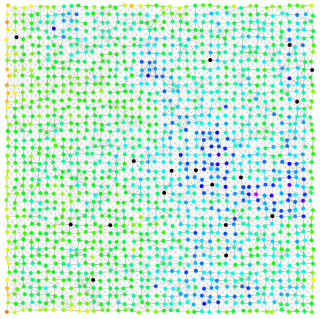
A grid of devices playing dodgeball

In this example we create a grid of devices and make them play dodgeball. The program to be injected is rather simple: some nodes will begin the simulation with a ball, and their goal will be to throw it to a random neighbor; whichever node gets hit takes a point, updates its score, and throws the ball again. This program is easy to write in a network of programmable tuple spaces, hence we write the following specification using the SAPERE incarnation.

Click to show / hide code

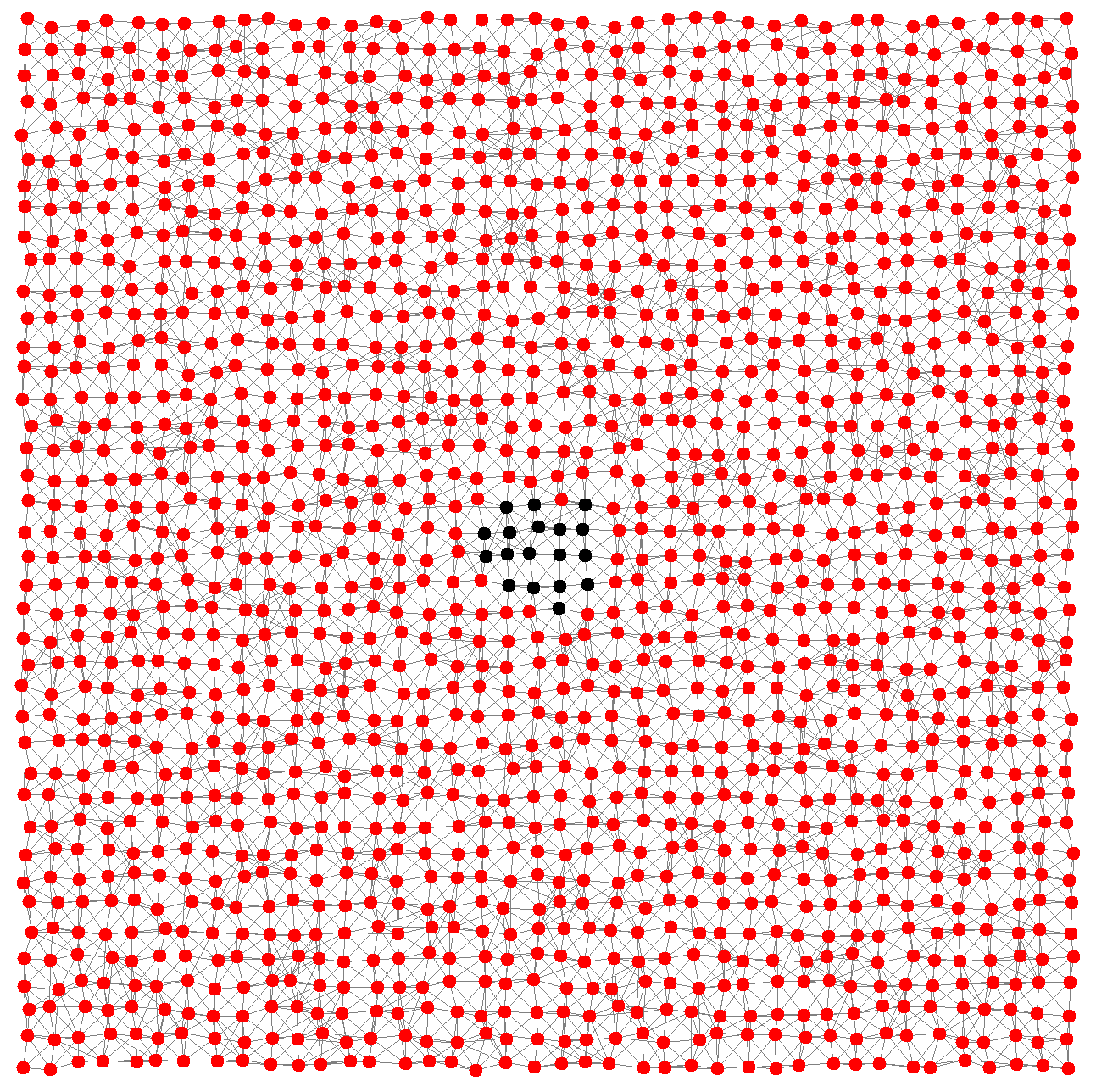
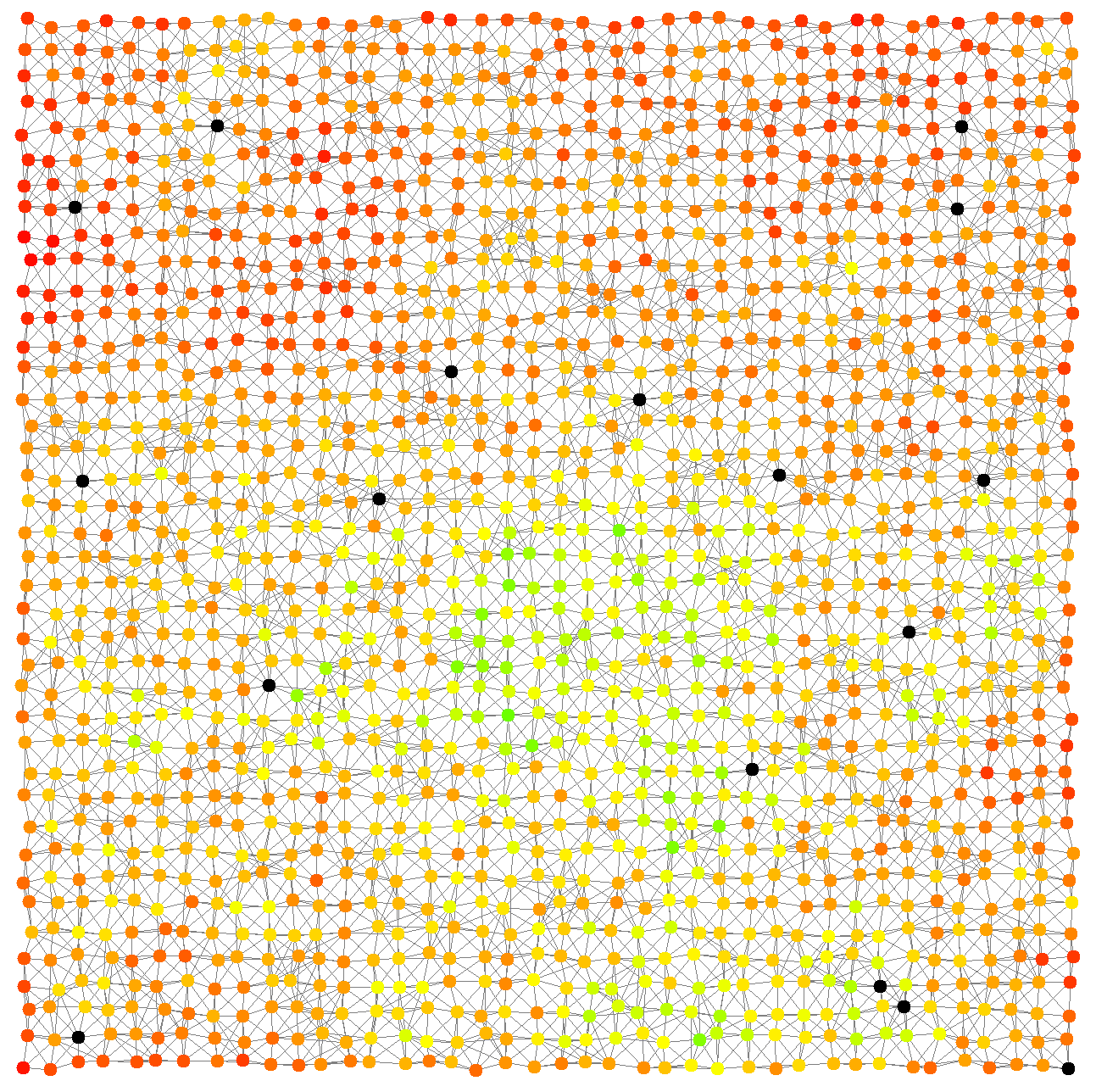
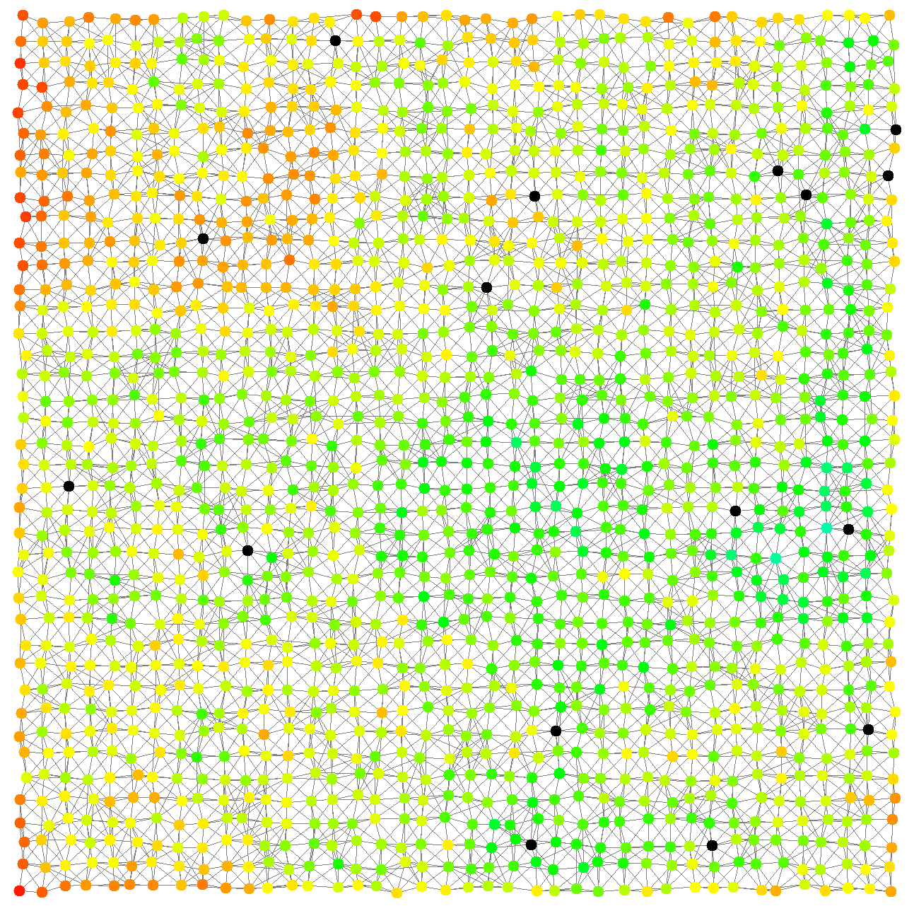
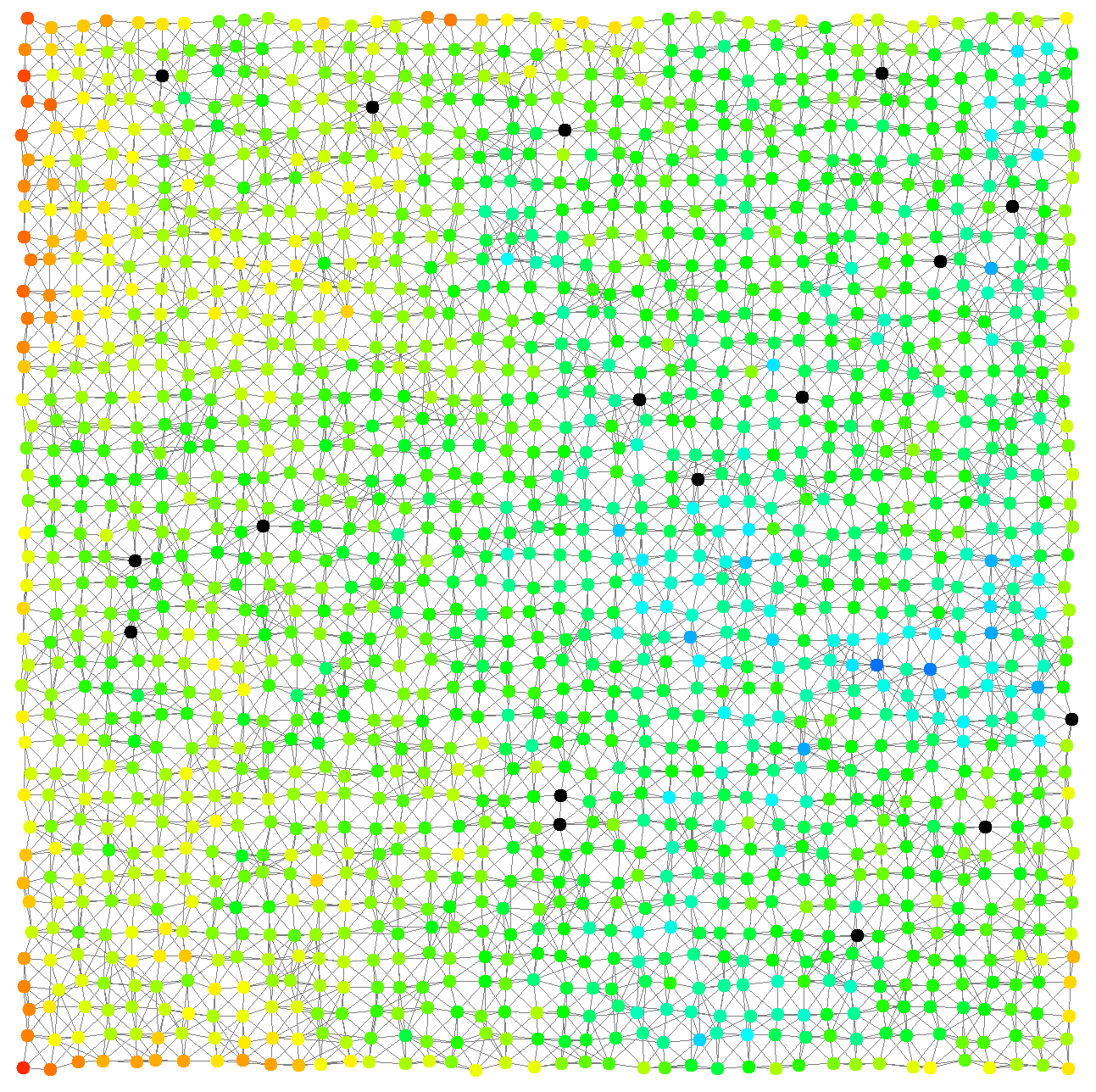
Snapshots of the simulation of the “dodgeball” example follow. Devices with a ball are depicted in black. All other devices’ color hue depends on the hit count, shifting from red (zero hits) towards blue.

Show snapshots

Dodgeball Dodgeball Dodgeball Dodgeball Dodgeball Dodgeball Dodgeball Dodgeball Dodgeball Dodgeball

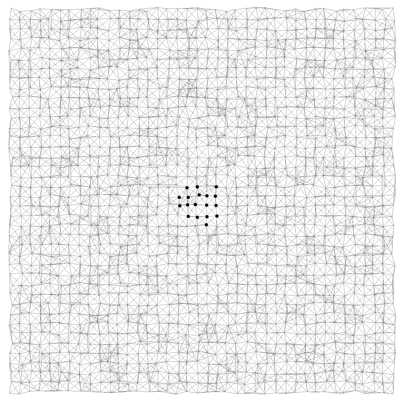
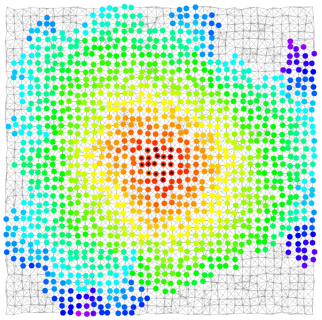
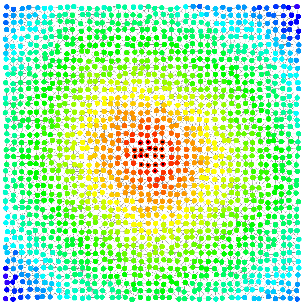
A gradient on a grid of devices

In this example, we implement with the SAPERE incarnation a very simple specification of a gradient, a pattern that is considered to be the basis of many other patterns 1

Click to show / hide code

Here are some snapshots of the simulation of the “gradient” example. Source devices have a central black dot. Devices’ color hue depends on the gradient value, shifting from red (low) towards blue (high).

Show snapshots

Gradient Gradient Gradient Gradient Gradient Gradient

Arbitrary network graphs

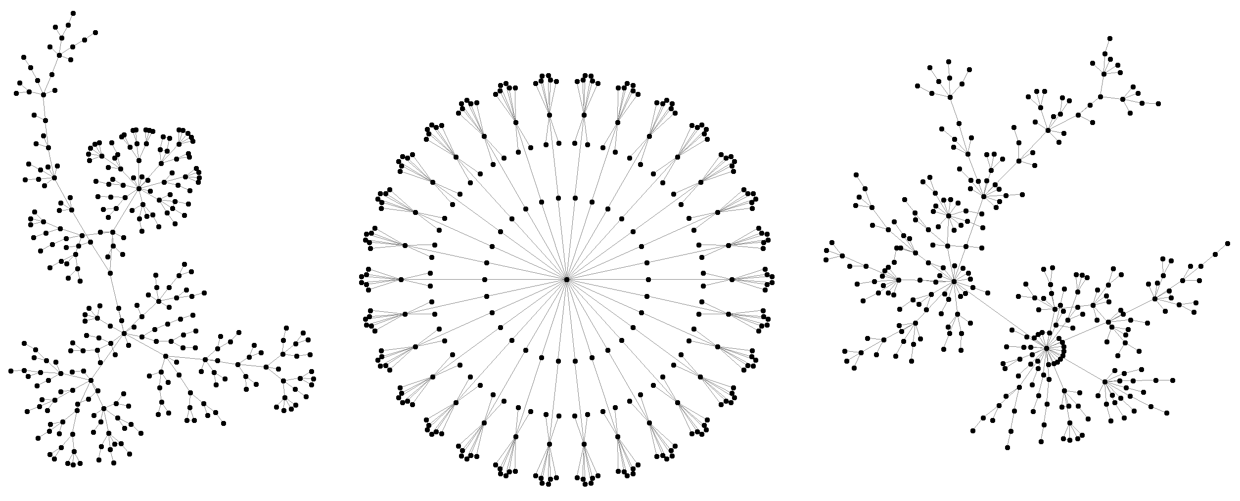
This example showcases some complex deployments made possible by Alchemist via Graphstream

Click to show / hide code

The example creates a single environment with three advanced deployments. From left to right: a Lobster graph, a banana tree, and a scale-free network with preferential attachment.

Arbitrary graphs Arbitrary graphs

Advanced examples

In this video, we learn how to:

  1. use aggregate programming (via Protelis) to write simulations;
  2. use images to create indoor environments with physical obstacles;
  3. use OpenStreetMap data to simulate on real-world maps; and
  4. export data from simulations and configure batches exploring all possible combinations

Node mobility and indoor environments

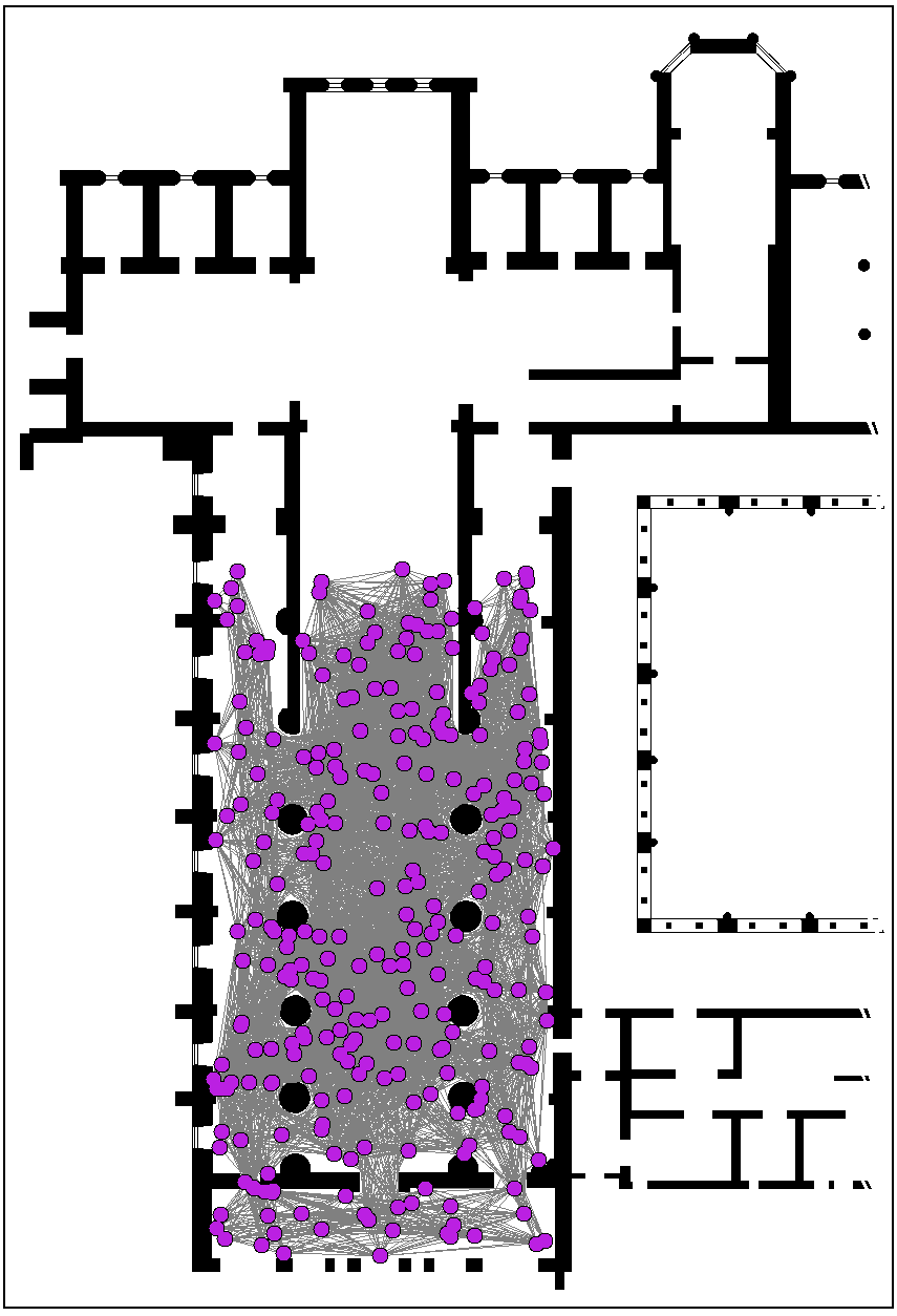
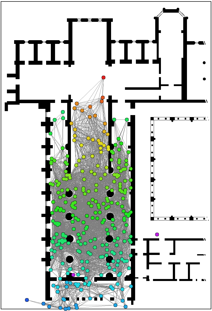
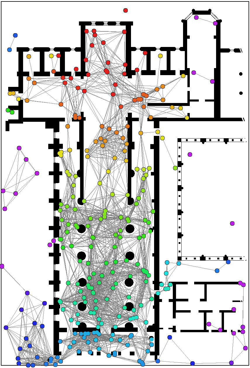
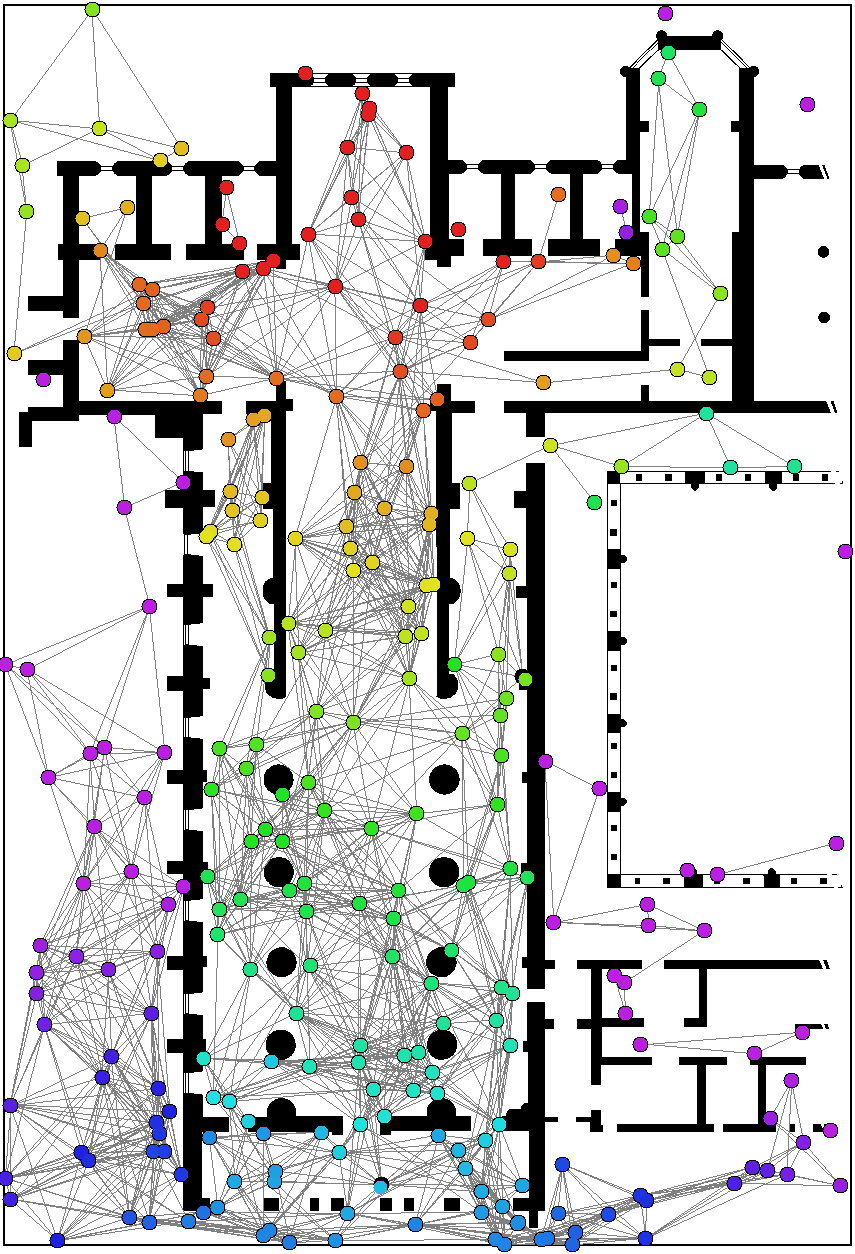
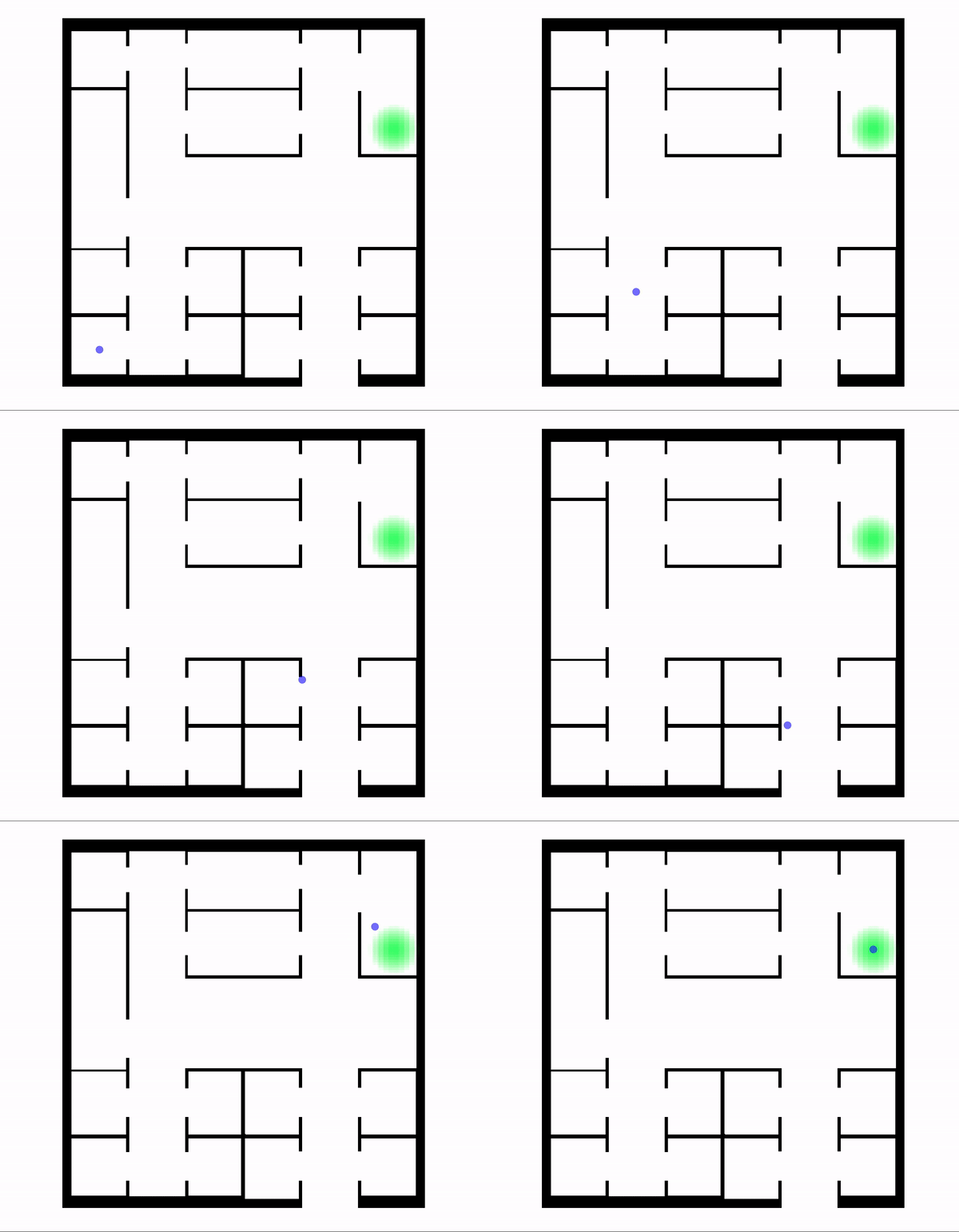
Many interesting scenarios the simulator targets require mobility and a richer environment. In the following example, we show a group of mobile devices estimating the distance from a point of interest (the altar) while moving within a church, whose planimetry has been taken from an existing building. Since the gradient is propagated in a network of mobile devices, we use a Protelis implementation of the adaptive Bellman-Ford algorithm from the Protelis-lang library2

Click to show / hide code

In the following snapshots, mobile devices progressively explore the location, while measuring the distance from a point of interest via gradient (red nodes are closer to the point of interest; purple ones are farther).

Show snapshots

Mobility in indoor environments Mobility in indoor environments Mobility in indoor environments Mobility in indoor environments Mobility in indoor environments Mobility in indoor environments Mobility in indoor environments Mobility in indoor environments

Real-world maps and GPS traces

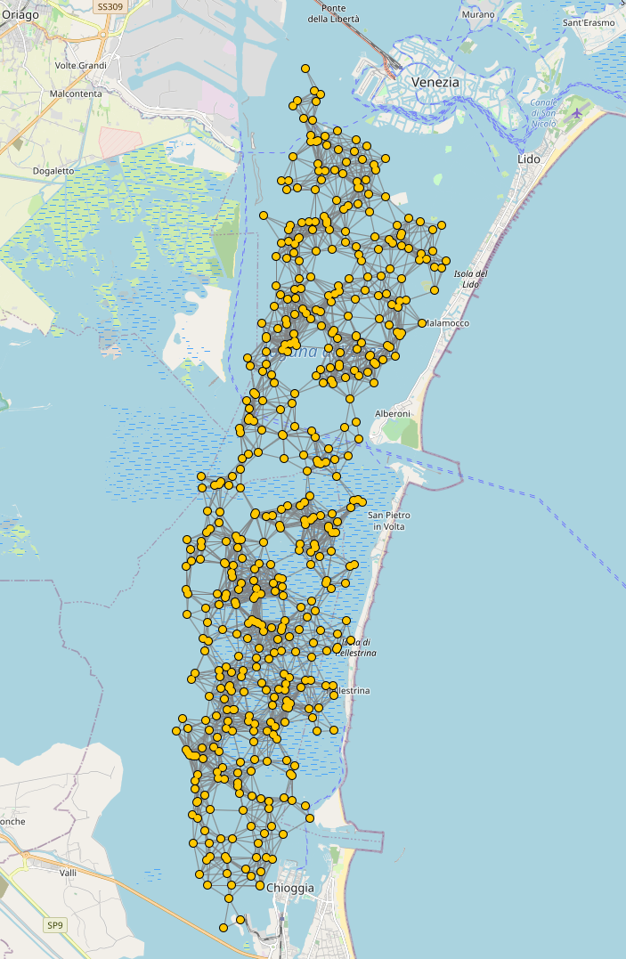
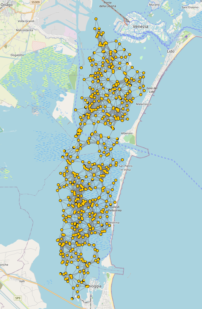
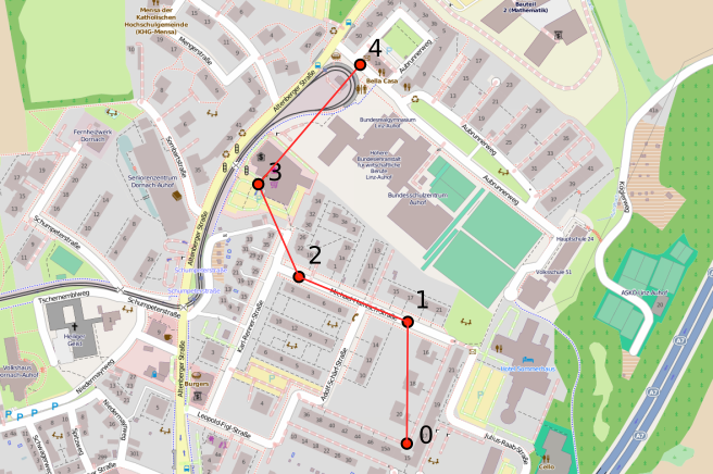
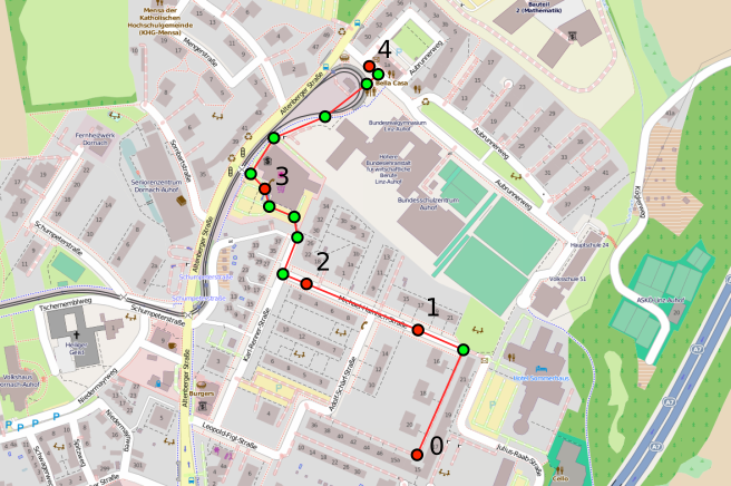
The simulator can load data from OpenStreetMap exports, navigate devices towards a destination along streets by relying on GraphHopper or by using GPS traces in GPX format, or even using the navigation system to interpolate sparse GPS traces, thus preventing nodes from taking impossible paths. In the following simple scenario buoys are deployed in the Venice lagoon and move Brownianly.

Click to show / hide code

The following snapshots depict the simulation in execution.

Show snapshots

Venice Venice Venice Venice

In-depth analysis of simulated scenarios

The following snippet showcases the aforementioned features by enriching the example of a gradient in an indoor environment presented previously with:

  1. variables for the pedestrian walking speed, pedestrian count, and random seed;
  2. constants to ease the configuration of the simulation;
  3. a Kotlin resource search expressed as a variable;
  4. controlled reproducibility by controlling random seeds;
  5. export of generated data (time and several statistics on the gradient).
Click to show / hide code
Info

  1.  ↩︎

  2.  ↩︎

Protelis Incarnation Tutorial

Protelis, from the Latin word figuratively meaning “regarding a team”, is a language targeting the aggregate of devices rather than the single one. It has been developed on the solid foundation of Field Calculus, a theoretical model of aggregate programming, and it is written and interoperable with Java.

Learning Protelis

The language and all the machinery of Protelis are out of the scope of this tutorial. However, we warmly recommend to read this paper first, and then to deepen your knowledge of Protelis by reading the resources available in the official Protelis website.

A tutorial similar to the base tutorial, with increasingly rich examples and focused on the Protelis incarnation can be found on GitHub. The README.md file of the project explains the use and the steps to follow.

Note

Something went wrong along the line? Drop us an issue report and we’ll get back to you.

SAPERE Incarnation Tutorial

An explanation of the basics of the SAPERE Incarnation is available here. A tutorial similar to the base tutorial, with increasingly rich examples, focused on the SAPERE incarnation. Reference descriptions of the SAPERE LSA language inside the simulator are available here

The tutorial can be found on GitHub. The README.md file of the project explains the use and the steps to follow.

Show README.md
Note

Something went wrong along the line? Drop us an issue report and we’ll get back to you.

LSAs

Syntax details are available in the reference. The following code creates an irregular grid of devices, of which those located around the center of such grid contain the tuple { token }:

The relevant part here is molecule: token. If we wanted to inject the tuple { foo, 1, bar, 2 }, we could have written molecule: foo, 1, bar, 2.

Eco-Laws

Nodes can be programmed with Eco-Laws as follows:

Eco-Laws can be programmed to send LSAs to neighbors, as well as to look into neighboring nodes for getting LSAs. In order to do so, the LSA template in the Eco-Law must be preceded by a neighbor operator, either + or *.

+ means in a neighbor: if used on the left hand side, it considers the condition satisfied if at least one neighbor has at least one LSA matching the provided template; if used on the right hand side, sends the LSA to one random neighbor.

* means in all neighbors: if used on the left hand side, it considers the condition satisfied if all neighbors have at least one LSA matching the provided template; if used on the right hand side, sends a copy of the LSA to all neighbors.

The following code exemplifies a diffusion program: when { token } is present locally, it is copied into neighboring nodes once per second; and as soon as two copies of { token } are present, one gets removed.

Rates

The time distribution with which reactions should get scheduled can be controlled by thinkering with the yaml specification as per every reaction in Alchemist. If no TimeDistribution is specified, the Eco-Law is assumed to run “as soon as possible” (ASAP).

This may lead to unwanted behaviour. For instance, programming a single node with: --> { foo } will cause the simulation to schedule a reaction producing { foo } at time zero, and at each execution the time will remain zero: the simulator will be producing copies over copies of the tuple, never advancing in time (Alchemist is a discrete event simulator), and possibly going on until the JVM memory limit is reached.

If a number is specified as time distribution, using the time-distribution key, then it will be interpreted as the Markovian rate of an exponentially distributed time.

Other distributions found at it.unibo.alchemist.model.timedistributions can be used leveraging the arbitrary class loading system.

In the following example, two Eco-Laws are configured, and one of them is bound to an ExponentialTime with rate 1, namely, when the reaction can be executed (the left hand LSAs have local matches), it will execute at an average of once per second (with a variance of 1 s²).

Exercise

To better grasp details of the incarnation, we recommend looking at the examples available on the Alchemist SAPERE Incarnation tutorial on GitHub.

Besides examples with growing complexity, there are a number of proposed exercises that should help you get acquainted with the SAPERE way of writing self-organizing behaviors.

Scafi Incarnation Tutorial

ScaFi (Scala Fields) is a Scala-based library and framework for Aggregate Programming. It implements a variant of the Higher-Order Field Calculus (HOFC) operational semantics, which is made available as a usable domain-specific language (DSL), and provides a platform and API for simulating and executing Aggregate Computing systems and applications.

How to use ScaFi with Alchemist

For more details about ScaFi please read the documentation in the official site where you can find a description of how to integrate ScaFi toolkit with Alchemist.

A tutorial similar to the base tutorial, with increasingly rich examples, focused on the Scafi incarnation.

The tutorial can be found on GitHub. The README.md file of the project explains the use and the steps to follow.

Simulations with Alchemist and Scafi: tutorial

This tutorial presents a sequence of increasingly rich examples using the Scafi aggregate programming DSL and the Alchemist Simulator.

Requirements

Check if it works

Open a terminal and type

java -version
git --version

Now you are ready to launch Alchemist & ScaFi simulations

Quickstart

Open a terminal and run:

Windows

curl https://raw.githubusercontent.com/scafi/learning-scafi-alchemist/master/launch.ps1 | Select-Object -ExpandProperty Content | powershell.exe

Linux & Mac

curl https://raw.githubusercontent.com/scafi/learning-scafi-alchemist/master/launch.sh | bash

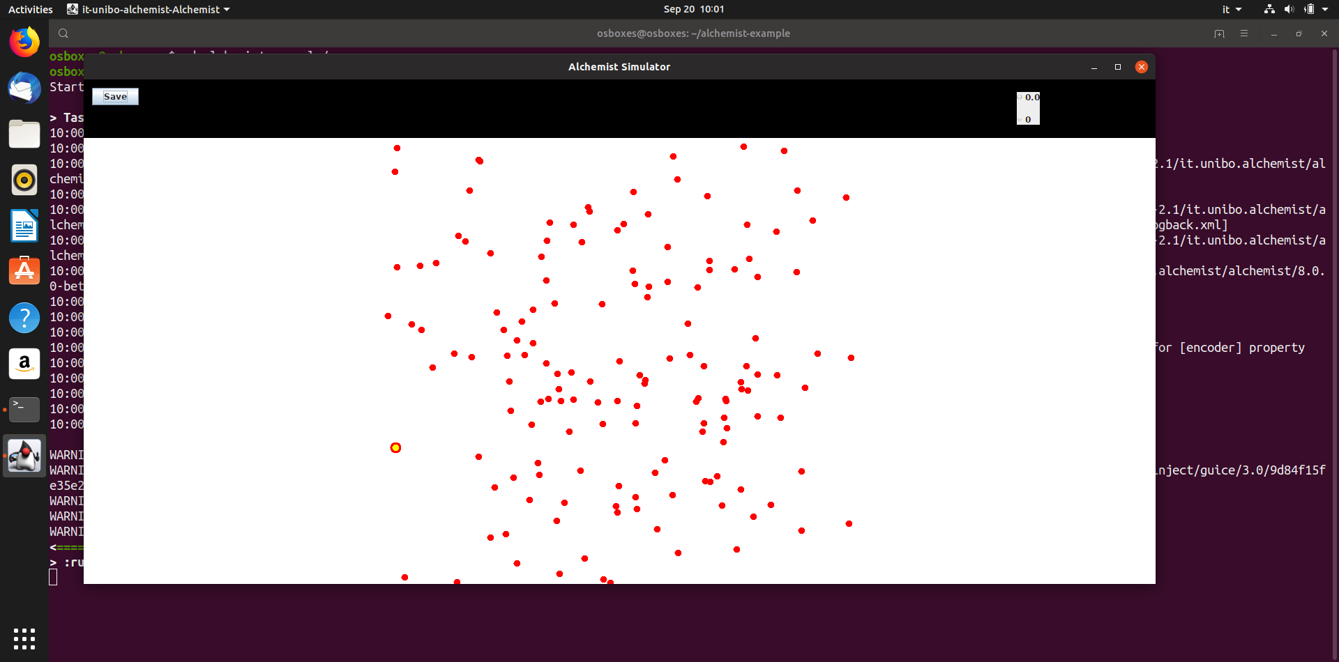
It will take some time for the system to download all the required dependencies, at the end of the process you will be presented the Alchemist default GUI (here are instructions on how to interact with the simulator). At this point, the simulation should be looking like this: Alchemist simulation start Alchemist simulation start

Click P to start the simulation. The nodes will compute the ScaFi program described here) in rounds, producing node colour changes. Alchemist simulation evolution Alchemist simulation evolution

What happened

Issuing the one-liner command, you have:

  1. downloaded this repository using Git
  2. created a folder called learning-scafi-alchemist that contains the simulations
  3. executed the command ./gradlew runHelloScafi inside the learning-scafi-alchemist created above.

The last command produces the execution of the simulation called helloScafi described using a yml file. Particularly an Alchemist simulation typically consists of a network of devices that could communicate with each other by means of a neighbourhood relationship (you can see the connections by clicking L) Alchemist Neibourhood Relationship Alchemist Neibourhood Relationship In this case, the nodes’ positions are configured through real GPS traces from the Vienna marathon app. The simulation effects (i.e., node shapes and colours) are highly configurable through JSON configuration. Here the node colour depends on the output of the ScaFi program, which is executed in each device every 1 second. Particularly, the execution of a ScaFi program deals with local computations and interaction among neighbours through a distributed data structure called computational field. This distributed and repeated execution of rounds eventually produces a collective result (you can find more details about the execution model of ScaFi programs in the documentation).

In this case, the program consists of the evaluation of the distance from the node with the ID 100 (in Aggregate Computing literature called “gradient”).

Something wrong?

Try the following:

  1. clone manually using git clone https://github.com/scafi/learning-scafi-alchemist.git
    1. alternatively: download the repository zip (Download!)
    2. then unzip the repository to a local folder
  2. open a terminal inside the cloned/downloaded folder
  3. run ./gradlew runHelloScafi

If you still have problems executing the experiments, please consider opening an issue! New issues

Guided examples

from now on, we will assume all commands have been issued inside learning-scafi-alchemist

1. Hello, ScaFi! A gradient in space and time

Launch command

./gradlew runHelloScafi

What happened

This is the example described in Quickstart section. Particularly, the program consists of the description of the self-healing gradient: an algorithm that computes a gradient (i.e., a field mapping each device in the system with its minimum distance from the closest source device) field and automatically adjusts it after changes in the source set and the connectivity network (more details about gradients can be found in Compositional Blocks for Optimal Self-Healing Gradients).

What is inside

Configuration File ScaFi Program File
helloScafi.yml HelloScafi.scala

An Alchemist simulation could be described through yml configurations. In order to execute ScaFi script, you should at least define:

  • the Scafi incarnation:
incarnation: scafi
  • a Reaction that contains the Action RunScafiProgram with the full class name of the program chosen
_reactions:
  - program: &program
      - time-distribution:
          type: ExponentialTime
          parameters: [*programRate]
        type: Event
        actions:
          - type: RunScafiProgram
            parameters: [it.unibo.scafi.examples.HelloScafi, *retentionTime]
      - program: send
  • a deployment that contains in the programs the Action specified above
deployments: ## i.e, how to place nodes
  type: FromGPSTrace ## place nodes from gps traces
  parameters: [*totalNodes, *gpsTraceFile, true, "AlignToTime", *timeToAlign, false, false]
  programs: ## the reactions installed in each nodes
    - *program

More details about the Alchemist configuration could be found in the official guide.

The main logic of the node behaviour is described through the Scafi program file. Particularly, a valid ScaFi program must:

  1. choose an incarnation
import it.unibo.alchemist.model.scafi.ScafiIncarnationForAlchemist._
  1. extend the AggregateProgram trait
class HelloScafi extends AggregateProgram
  1. mix-in the libraries required for the application
with StandardSensors with ScafiAlchemistSupport with BlockG with Gradients with FieldUtils {
  1. define the behaviour inside the main method.

A ScaFi program typically deals with environment information through sensors. sense[Type](name) is the built-in operator used to query the sensors attached to each node. Each molecule expressed in the yaml (i.e., the Alchemist variable concept) can be queried from the ScaFi program. For instance, in helloScafi, we write:

- molecule: test
  concentration: *source # anchor to "source" value, check line 17

Therefore, in the program, we can get the test value as:

// Access to node state through "molecule"
val source = sense[Int]("test") // Alchemist API => node.get("test")

There are several built-sensors (in checkSensors there are examples of local sensors and neighbouring sensors). For more details, please check the Scaladoc.

The main logic of the program is expressed in the following line:

// An aggregate operation
val g = classicGradient(mid() == source)

Where classicGradient is a function defined in BlockG that implements the self-healing gradient described above. The first argument is a Boolean field that defines which part of the system could be considered a source zone. In this case, nodes are marked as source when the field of ids (i.e., mid()) is equal to the value passed through the variable test. This can be expressed as mid() == source.

The value produced by Scafi definitions could be used to express actuation. In the Scafi incarnation, you can update the Alchemist variables through node.put

// Write access to node state (i.e., Actuation => it changes the node state)
node.put("g", g)

In the Alchemist default GUI you can inspect the node variables (i.e., molecules) by double-clicking a nodes Alchemist Molecule panel Alchemist Molecule panel

Finally, the last instruction of the main is the returned value of the Scafi program (in scala return is optional)

// Return value of the program
g

Minimal changes

  1. As described above, the program is self-healing, so try to move node and see how the system eventually reaches a stable condition:
    • click S to enter into selection mode
    • start a selection by clicking the mouse left button and dragging it into the environment
    • once your selection is over, click O to enter into move mode
    • click over the selection and drag the element into another position Alchemist Move elements Alchemist Move elements
  2. Try to modify the source node (via yml configuration) and check the program output differences
  3. Try to change the source node (i.e. with the ID == 10) after 10 seconds (check BlockT library, or you can implement the time progression with rep(0 seconds)(time => time + deltaTime))

Using the generated data with the embedded plotting script

You can produce plots from the data generated by Alchemist simulations. Indeed, each Alchemist simulation produces aggregated data as expressed in the export configuration section. For more details about data exporting, please refer to the official Alchemist guide.
Particularly, this command:

./gradlew runHelloScafi -Pbatch=true -Pvariables=random

will run several simulations in batch, one for each possible value of the random variables (six in this case, as expressed in the helloScafi.yml). Each simulation, will produce a csv file in $exportPath/$fileNameRoot-randomValue.$fileExtension (in this case, build/exports/helloScafi/experiment-x.txt, the values starting with $ are gathered from the simulation configuration file).

Typically, we use these data to produce charts that express the dynamics of the collective system. This repository contains a highly configurable script (please look at the configuration defined in plots).

To run the script for this experiment, you should run:

$ python plotter.py plots/helloScafi.yml ./build/exports/helloScafi ".*" "result" plots/ 

Where:

  • the first argument is the plot configuration (expressed using a yaml file)
  • the second argument is where the files are located
  • the third argument is a regex used to select the simulations file
  • the fourth argument defines the initial names of the plot
  • the last argument devises the folder in which the plots will be stored

2. A richer pattern: Self-organizing Coordination Regions

Launch command

./gradlew runSelforgCoordRegions

What happened

This example shows an interesting pattern developed with ScaFi, the so-called Self-Organising Coordination Regions (SCR). (more details in Self-organising Coordination Regions: A Pattern for Edge Computing)

The idea of SCR is to organize a distributed activity into multiple spatial regions (inducing a partition of the system), each one controlled by a leader device, which collects data from the area members and spreads decisions to enact some area-wide policy. Particularly, when you launch the command of SCR you will see something like this:

SCR result SCR result

Where the colour denotes the potential field (i.e., the gradient) that starts from the selected leader. In this GIF, the leaders are the ones marked with blue colour.

What is inside

Configuration File ScaFi Program File
selforgCoordRegions.yml SelforganisingCoordinationRegions.scala

The SCR pattern consists of four main phases:

  1. leader election: using block S the system will produce a distributed leader election that tries to divide the system equally with a certain range (in S term, it is called grain):
// Sparse choice (leader election) of the cluster heads
val leader = S(sense(Params.GRAIN), metric = nbrRange)
  1. potential field definition: after the leader election process, there is another phase in which will be computed potential field from the leader. In this way, the slave node could send information to leader’s
// G block to run a gradient from the leaders
val g = distanceTo(leader, metric = nbrRange)
  1. collection phase: the slave node could collect local information (e.g., temperature) and send it to the leader. During the path, it will be an aggregation process that combines local information with area information (i.e., all the nodes that are inside the potential field of a leader)
// C block to collect information towards the leaders
val c = C[Double,Set[ID]](g, _++_, Set(mid()), Set.empty)
  1. leader choice and share: with the information collected inside an area, the leader could perform an area-wide decision and then send it to the whole area (using G)
// G block to propagate decisions or aggregated info from leaders to members
val info = G[Set[ID]](leader, c, identity, metric = nbrRange)
val head = G[ID](leader, mid(), identity, metric = nbrRange)

Minimal changes

  1. Try to change the grain (check in the configuration file). It would lead to changes in area formation
  2. Try to count the number of nodes inside an area and share this information with that area—suggestion: change phase 3. of the SCR
  3. As in the previous example, the areas are self-healing. Therefore try to move leaders and see what happens in the leader formation. Try to remove nodes too (see the next clip) ezgif com-gif-maker ezgif com-gif-maker

3. Overlapping computations in space and time with aggregate processes

./gradlew runAggregateProcesses

What happened

This example shows an application of Aggregate Processes, which is s a way to specify a dynamic number of collective computations running on dynamic ensembles of devices (more details in Engineering collective intelligence at the edge with aggregate processes). Processes API Processes API

The processes are the bigger circle around the nodes. The colour identifies the process ID. As you can see, during the simulation the process starts, shrink and then could disappear.

What is inside

Configuration File ScaFi Program File
aggregateProcesses.yml SelforganisingCoordinationRegions.scala

Minimal changes

To start the process, you can use the spawn operators (and their variation, sspawn, cspawn, etc.):

val maps = sspawn[Pid,Unit,Double](process, pids, {})

Particularly, sspawn accepts:

  • the process logic, that is a function ID => Input => Pout[Out]
    • ID in this case is a case class that contains the id of a node that will start the process, the time in which it will effectively start and finally the time in which it will end.
    case class Pid(src: ID = mid(), time: Long = alchemistTimestamp.toDouble.toLong)
                  (val terminateAt: Long = Long.MaxValue)
    • The input of the process (in this case is empty)
    • Finally, the Pout[Double] is the process output. Pout is a data structure that contains the output of the process and the status of the process (that could be Output, Terminated and External—more details in the paper).
  • The key set of the process that will be spawn (pids)
    • In this case, the new pids associated to new processes are selected from Alchemist molecule.
    def processesSpec: Map[Int,(Int,Int)] = sense(MOLECULE_PROCS)
    • From this information il will be created the pids for the processes:
    // Determine the processes to be generated (these are provided in a molecule "procs")
    val procs: Set[ProcessSpec] = processesSpec.map(tp => ProcessSpec.fromTuple(tp._1, tp._2)).toSet
    val t = alchemistTimestamp.toDouble.toLong
    val pids: Set[Pid] = procs.filter(tgen => tgen.device == mid() && t > tgen.startTime && (t - 5) < tgen.startTime)
      .map(tgen => Pid(time = tgen.startTime)(terminateAt = tgen.endTime))

Particularly, in this case, the process logic is quite simple:

  • it produces a potential field from the processes creator
  • it terminates if the terminateAt is reached
  • the nodes that belong to nodes are the ones that are inside the bubble, that is the nodes inside an area of 200 units
def process(pid: Pid)(src: Unit = ()): POut[Double] = {
  val g = classicGradient(pid.src==mid())
  val s = if(pid.src==mid() && pid.terminateAt.toDouble <= alchemistTimestamp.toDouble){
    Terminated
  } else if(g < 200) Output else External
  POut(g, s)
}

Minimal changes

  • Try to add the extension of the bubble as a parameter (as the start and end time)
  • Even in this case, the computation is self-healing. Therefore, try to move the process center to see how the system reacts
  • Try to add other processess (see the yaml configuration)

External resources to improve your understanding

Note

Something went wrong along the line? Drop us an issue report and we’ll get back to you.

How-to Guides

Problem-oriented

How-to Guides

Contents

Subsections of How-to Guides

Preparation

Set up the simulation environment

Preparation

Contents

Subsections of Preparation

Alchemist stand-alone

Although we recommend to run the simulator via Gradle, Alchemist can be executed through the redistributable jar file.

Such jar file can be downloaded from the releases section on github.

Obtain the runnable jar of alchemist-full from GitHub, the open a terminal and move to the folder where the jar is located, then issue:

java -jar alchemist-full-VERSION-all.jar --help

Remember to substitute VERSION with the Alchemist version you actually have downloaded. You can still use alchemist in a modularized form using jars. In this case, use alchemist-VERSION-all.jar and all the jars corresponding to the modules you need. Pass them to the java command as classpath, e.g.:

java -cp alchemist-VERSION-all.jar:alchemist-incarnation-protelis-VERSION-all.jar:alchemist-swingui-VERSION-all.jar it.unibo.alchemist.Alchemist --help

Under Windows, the separator is ; in place of :

This command will print information on the available command line options.

Simulation

Prepare the simulated environment

Simulation

Contents

Subsections of Simulation

Create reusable variables

Declaring variables

The variables section lists variable simulation values. A variable defines some kind of value that can be referenced in the simulation file.

There are two kinds of variables: free and dependent variables. Free variables are meant to provide support for running batches of simulations with varying parameters; dependent variables are either single valued or can be computed from the values of other variables (free or dependent), and they are designed to simplify the simulation code.

Free variables

Free variables define a set of values and a default. Their main scope is enabling Alchemist to run a set of simulations with different parameters (values of variables) without the need to duplicate the simulation code. When used in this mode (called “batch mode”), Alchemist by default produces the cartesian product of all the variables values’ selected for the batch, and runs a simulation for each combination. If the simulation is not executed as batch, then the default value is used.

Linear variables

A variable generating values in a range, starting from a minimum value, and increasing by some step. Represented by LinearVariable.

Examples

Click to show / hide code

Geometric variables

A variable generating geometrically-distributed samples across a range. Ideal for exploring non-linear phenomena, or for exploring very large ranges of values whose effect is unknown. Implemented as GeometricVariable.

Examples

Click to show / hide code

Arbitrary-valued variables

Generates an ArbitraryVariable spanning on an arbitrary set of values.

Examples

Click to show / hide code

Dependent variables

Some variables are combination of other variables. Let’s suppose that we want to deploy on a circle, but for some reason (e.g. because it is required by the constructor of some Action) we need to compute and have available radius and perimeter. We don’t need to control both of them: the perimeter can be computed from the radius (or vice versa).

To favor reusability and apply the DRY principle, the simulator allows defining variables whose values possibly depend on values of other variables through JSR223Variable. Their values can be expressed, by default, in Groovy, but any JSR-223-compatible language can be used, in principle. If a compatible JSR-223 implementation of the language is available in the classpath, Alchemist will load and use it transparently. By default, groovy, kotlin (or kts), and scala are available as scripting languages for dependent variables.

Info

The JSR-223 specification defines mechanisms allowing scripting language programs to access information developed in the Java Platform.

Many languages (including Groovy, Python (Jython), Kotlin, and Scala provide bindings for JSR-223).

Variables can be defined in any order. Alchemist figures out the dependencies automatically, as far as there are no cyclic dependencies (e.g. variable a requires b, and b requires a). Please note that the simulator variable dependency resolution system is not designed to solve mathematical systems, so even though the problem has a well-formed mathematical solution, the actual variable resolution may fail; e.g. if a is defined as 2 * b + 1, and b is defined as 4 - a, the system won’t bind a to 3 and b to 1, but will simply fail complaining about circular dependencies.

Multiline programs

Sometimes data manipulation can get tricky and trivial scripting may no longer be enough. In such cases, and especially with modern languages that allow for a reduced usage of cerimonial semicolons (such as Kotlin and Scala), it can be useful to write multiline programs. This can be achieved in YAML by using the pipe | operator, as exemplified in the following snippet:

multiline-string: |
  note that the string
  needs to be indented.
  Newlines will be preserved!  

Examples

Click to show / hide code

Ensure repeatability

Debugging a simulation requires the ability to reproduce the same behavior multiple times: an unexpected behavior requiring investigation may happen far into the simulation, or in corner conditions encountered by chance. Randomness is controlled by setting the random generator seeds separately for the deployments and the simulation execution, allowing for running different simulations on the same random deployment.

Alchemist simulations can be reproduced by feeding them the same random number generator. This assumption is true as far as the custom component in use:

  • do not use any other random generators but the one provided by the simulation framework (all the standard components are guaranteed to do so);
  • do not iterate over collections with no predicible iteration order (e.g., Java’s Set and Map) containing elements (or keys) whose hashCode() has not been overridden to return the same value regardless of the specific JVM in use;
  • do not run operations in parallel.

The seeds section control the random generation process and may contain two optional values: scenario and simulation. The former is the seed of the pseudo-random generator used during the creation of the simulation, e.g. for deploying nodes in random arrangements. The latter is the seed of the pseudo-random generator used during the simulation, e.g. for computing time distributions or generating random positions. A typical example in which one may want to have different values, is to keep the same random deployment of devices in some scenario but allow events to happen with different timings.

Click to show / hide code

Usually, in batches, you wan to run multiple runs per experiment, varying the simulation seed, in order to get more reliable data (and appropriate error bars). As per any other value, variables can be feeded as random generator seeds.

Cognitive Agents

We recommend to read our explanation of the cognitive agents to better understand the contents of this how-to.

Different kinds of pedestrians are obtainable by attaching NodePropertys to nodes (e.g GenericNode). Common properties concern abilities such as perceiving other nodes (PerceptiveProperty) and occuping space in an environment (OccupiesSpaceProperty).

Homogeneous Pedestrian

As shown in the example below, this kind of pedestrian is obtained by attaching the Pedestrian property.

Click to show / hide code

Heterogeneous Pedestrian

The age groups available are: child, adult, and elderly; alternatively, if the exact age is specified, they are assigned to one of the aforementioned groups automatically. The genders available are: male and female. This informations is included in the Human property and it is used by the HeterogeneousPedestrian property, along with the age.

Click to show / hide code

Cognitive Pedestrian

Cognitive pedestrians are heterogeneous pedestrians with cognitive capabilities given by a CognitiveProperty. They have an emotional state and are able to influence and be influenced by others with the same capabilities. As an example, cognitive pedestrians can perceive fear via social contagion (e.g. seeing other people fleeing may cause them flee as well despite they haven’t directly seen the danger). To express how a cognitive pedestrians move, based on their emotional state, attach the CognitivePedestrian property.

Click to show / hide code

Homogeneous orienting pedestrian

These are homogeneous pedestrians that can be equipped with a given knowledge degree of the environment. Such quantity is a Double value in [0,1] describing the percentage of environment the pedestrian is familiar with prior to the start of the simulation (thus it does not take into account the knowledge the pedestrian will gain during it). Note that despite their name (“homogeneous”), knowledge degrees of different homogeneous orienting pedestrians may differ, and even pedestrians with the same knowledge degree can be different as each one can be familiar with different portions of the environment. Be also aware that orienting pedestrians can only be placed in an EnvironmentWithGraph which is a type of environment providing a navigation graph. In order to give a node orienting capabilities enhance a node with an OrientingProperty.

Click to show / hide code

Cognitive orienting pedestrian

These are cognitive pedestrians equipable with a given knowledge degree of the environment.

Click to show / hide code

Groups

It is likely that a pedestrian doesn’t move on its own, but there is a group consisting of multiple people which are related each other and whose behaviors are strictly dependent on that structure. The only way you can currently assign a group to a pedestrian is by creating it as a variable and passing it as a parameter when the Nodes created are of pedestrian type. If you don’t specify any group in this phase, automatically a new group of type Alone is assigned.

The following simulation example loads two groups of homogeneous pedestrians representing friends around the center of the scene, one having 10 members and the other 15.

Click to show / hide code

Steering Actions

Steering actions are Actions whose purpose is moving a node inside an environment. These actions can be divided into two categories:

  • greedy, i.e. performing only local choices;
  • NavigationActions, which exploit the spatial information available to orienting pedestrians in order to navigate the environment consciously (e.g. without getting stuck in U-shaped obstacles).

For a complete overview of the available actions refer to the api documentation. The creation of complex movements can be accomplished by combining different steering actions together. The only way currently available to do so is by using some SteeringBehavior extending Reaction, which can recognize, across all the actions specified, the steering ones to trait them in a separate way.

In this simulation 50 people wander around the environment and, if they are approaching an obstacle, they avoid it.

Click to show / hide code

Steering Strategies

In order to decide the logic according to which the different steering actions must be combined, the concept of steering strategy has been introduced and related to it different reactions are available to be used with the aim of computing the desired route for the pedestrians. If you want a pedestrian to execute a single steering action at a time, PrioritySteering is a reaction which gives relevance only to the steering action whose target point is the nearest to the current pedestrian position. If you want a pedestrian to execute a movement considering multiple actions at a time, BlendedSteering weights them considering their target distance to the current pedestrian position. There is no limit to the number of steering actions which can be used together but some messy compositions can result in unpredictable behaviors, so pay attention.

In the example below a pedestrian reaches a point of interest, avoiding in the meantime to approach another position.

Click to show / hide code

Danger and evacuations

Pedestrians can be loaded in any kind of Environment but it is recommended to use PhysicsEnvironments since they have properties such as non-overlapping shapes which are advisable to be taken into consideration when working with a crowd. To specify the existence of a potential danger or a significative zone in general inside the environment you can use Layers. You must specify to any cognitive pedestrian the Molecule representing danger in the Environment, otherwise it won’t have the ability to recognize its presence.

In the following example, 100 adult females with cognitive capabilities get away from a zone in the environment where there is a potential danger.

Click to show / hide code

Hardcoded parameters

Here’s a list of all the hardcoded parameters.

Name Value Description
knownImpasseWeight 10 Weight assigned to known impasses (= areas with a single door). It’s usually a high value, allowing to avoid them.
toleranceAngle 45 degrees Used by SinglePrevalent, that linearly combines multiple steering actions (= multiple forces) assuming one of them is prevalent. Weights for the linear combination are determined so that the resulting force forms with the prevalent one an angle smaller than or equal to the tolerance angle. The prevalent force usually wants to move the pedestrian consciously, whereas other forces are more “greedy”. The purpose of the tolerance angle is allowing to steer the pedestrian towards the target defined by the prevalent force, while using a trajectory which takes into account other urges as well.
alpha 0.5 Used by SinglePrevalent, an exponential smoothing with this alpha is applied to the resulting force in order to reduce oscillatory movements.
maxWalkRatio 0.3 Used by SinglePrevalent. When the pedestrian is subject to contrasting forces the resulting one may be small in magnitude, hence a lower bound for such quantity is set to (maximum distance walkable by the pedestrian) * (this parameter) so as to avoid extremely slow movements.
delta 0.05 Used by SinglePrevalent. The weight assigned to disturbing forces is set to 1 and then iteratively decreased by delta until the resulting force satisfies the required conditions (see the api). This is similar to a gradient descent.

Physical pedestrians

Physical pedestrians are capable of pushing and bumping into each other. To express those physical interactions use a PhysicalPedestrian property.

Physical steering strategies

In order to work properly, physical pedestrians should be equipped with physical steering strategies. Such strategies define how steering actions (which are intentional) are combined with physical forces (which are mostly unintentional). At present, only PhysicalBlendedSteering and NavigationPrioritizedSteeringWithPhysics are available.

Here’s a simple code for loading a homogeneous pedestrian with physical properties with CognitiveAgentSeek and CognitiveAgentFlee:

Click to show / hide code

Create a network

Alchemist nodes can connect to each other and form a network.

The network-model key is used to load the implementation of LinkingRule to be used in the simulation, which determines the neighborhood of every node.

The key is optional, but defaults to NoLinks, so, if unspecified, nodes in the environment don’t get connected.

Omitting the key is equivalent to writing any of the following:

network-model:
  type: NoLinks
network-model:
  type: NoLinks
  parameters: []

Linking nodes based on their respective distance

One of the most common ways of linking nodes is to connect those which are close enough to each other. To do so, you can use ConnectWithinDistance, passing a parameter representing the maximum connection distance.

Note that such distance depends on the environment: while the definition of distance is straightforward for euclidean spaces, it’s not so for Riemannian manifolds, which is a fancy name to define manifolds such as the one typical of a urban map (you can roughly interpret it as a euclidean space “with holes”).

For instance, in case of environments using GeoPosition, the distance is computed in meters, so the distance between [44.133254, 12.237770] and [44.146680, 12.258627] is about 2240 (meters).

In the following example, nodes are connected when closer than a threshold:

Click to show / hide code

Create Layers

simulation with layer simulation with layer

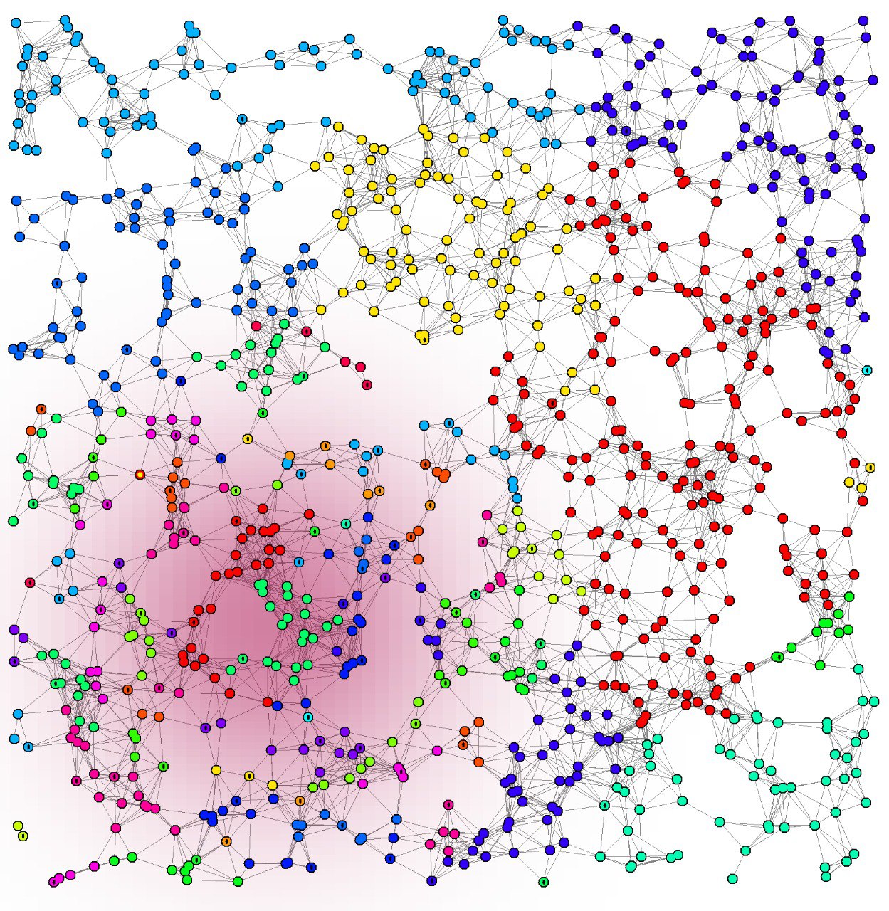
It is possible to define overlays (layers) of data that can be sensed everywhere in the environment. Layers can be used to model physical properties, such as pollution, light, temperature, and so on. As opposed to nodes’ contents, layers have no dependency optimization. This implies that reactions that read values from layers should have special care in defining their context appropriately.

Layers are created with the type/parameter syntax, as in this example:

Click to show / hide code

The following example shows the syntax for initializing multiple BidimensionalGaussianLayers:

Click to show / hide code

If the target layer is written in Kotlin, it can be loaded using named parameters, which arguably reads more clearly.

Click to show / hide code

Subsections of Create rich environments

Find paths indoors

The background regarding the navigation system is explained here.

Generating navigation graphs from images

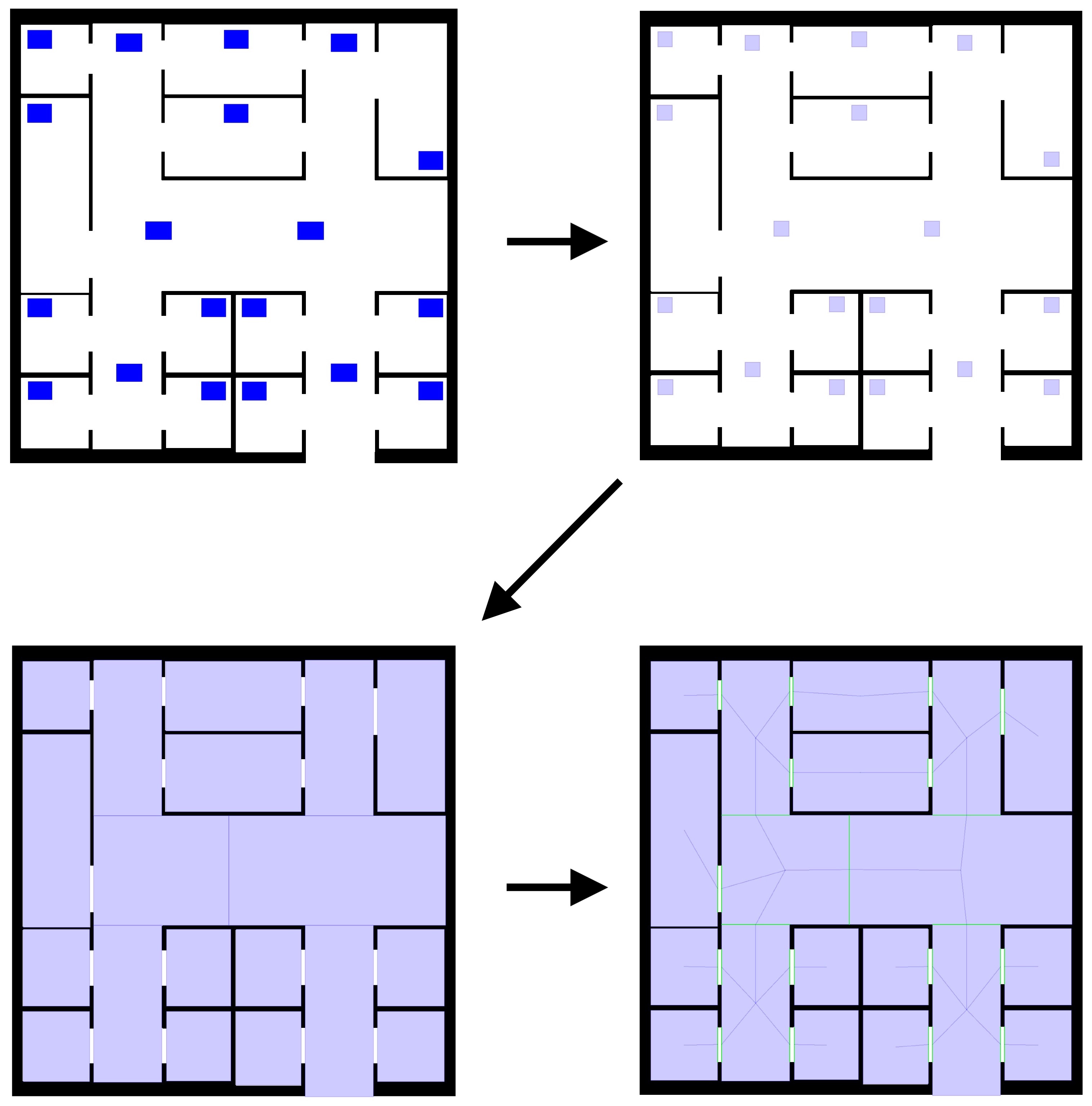
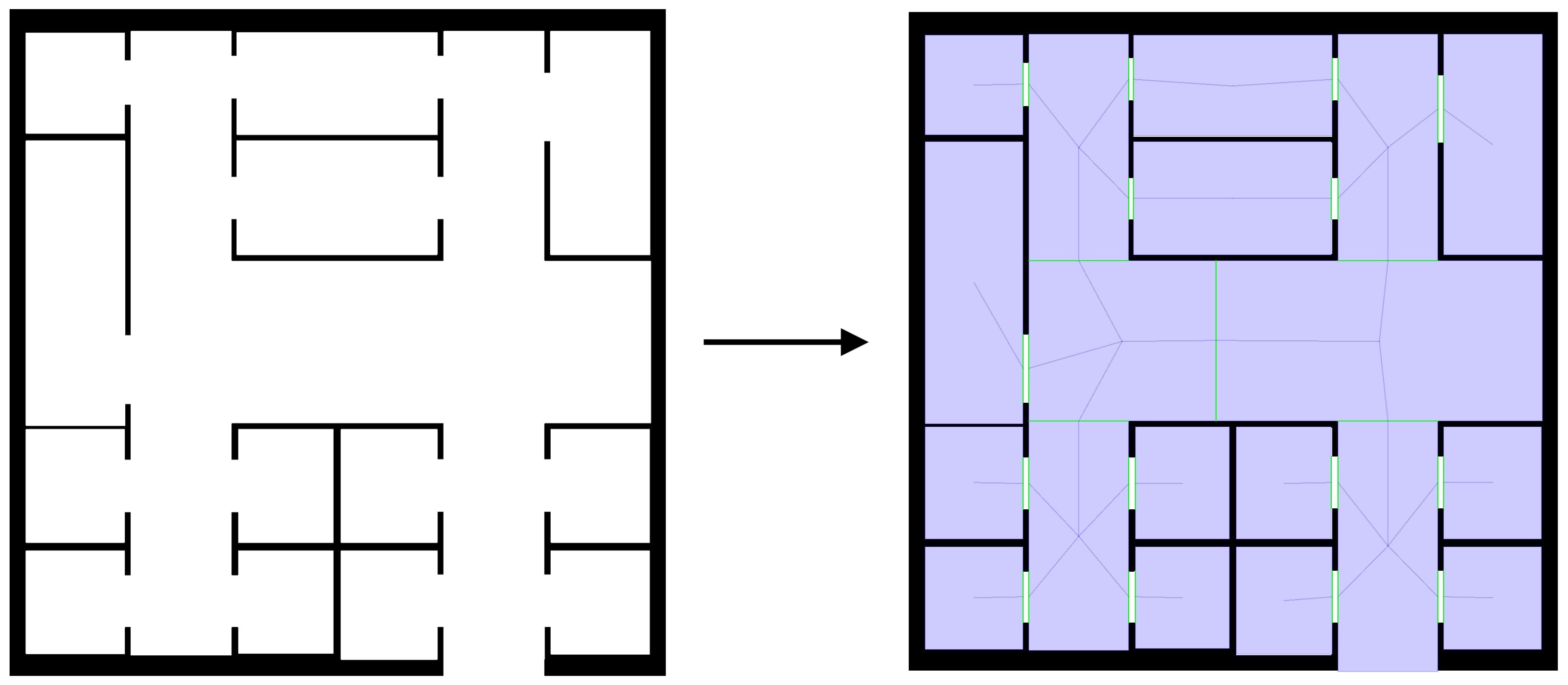
If your environment is codified as an image, generating a navigation graph is straight-forward. All you have to do is mark the areas of the environment where to plant initial seeds in blue (RGB #0000FF). In the image below you can see the generation of a navigation graph. The blue regions in the original image indicate where to plant initial seeds. These are then grown and crossings are found between them.

navigation graph generation navigation graph generation

Once you have your image ready for the generation of the navigation graph, you can exploit the ImageEnvironmentWithGraph class to produce it for you. This will read your image, extract the positions you marked blue and pass them to the NaviGator algorithm.

Examples

Click to show / hide code

Maps and GPS traces


Alchemist is equipped with the ability to load and simulate on real-world maps. Navigation on maps can be done by using gps traces, by moving along roads (Alchemist relies on GraphHopper to provide directions), by interpolating gps traces with on-the-road-movements, or by ignoring the map information and just move as you would in a continuous space.

Setting up a map environment

In order to run simulations on real world maps, an appropriate environment must be selected, such as OSMEnvironment.

If you need map data to perform on-streets routing, you need to feed it to the simulator. OSMEnvironment supports OpenStreetMap extracts in several formats, we recommend using the protocol buffer binary format (pbf) to save time and space.

OpenStreetMap extracts

It is likely that you do not need a simulation that requires navigation capabilities on the whole planet, especially considering that, even in binary format, it contains more than 50GB of data. We recommend thus to use an extract with the data relative to the area you are interested in simulating in. One great way to obtain an extract is through BBBike.

If you rely on their service, consider donating to the project.

Deploying nodes using GPS traces

We prepared a dedicated page on the argument

Navigate nodes in map environment

We prepared a dedicated page on the argument

Simulate indoor

indoor simulation indoor simulation

Indoor environments (bidimensional spaces with obstacles) can be generated from images by leveraging ImageEnvironment, which loads the map as raster image from file, interpreting the black pixels as obstacles (wall-like areas not accessible to nodes). Color of pixels that represents obstacles can be set to every color with a constructor’s parameter, black is default.

By default, each pixel is considered as a 1x1 block. As a consequence, a 1200x600 image with a vertical line of black pixels at coordinate 500 will be interpreted as a single obstacle of size 1x600 starting at coordinate (500, 0). It is possible to scale up or down the size of the environment by acting on the zoom parameter of ImageEnvironment, as well as changing the initial coordinates.

Examples

image from the project repository image from the project repository

Click to show / hide code

image from the project repository image from the project repository

Click to show / hide code

image from the project repository image from the project repository

Click to show / hide code

image from the project repository image from the project repository

  • Direct reference to the image
    Click to show / hide code
  • Search for the image in the file system via Kotlin
    Click to show / hide code

Simulate physical interactions among pedestrians

Before reading the following explanation you may want to look at the explanation of the cognitive agents and then at how to work with them.

Configuring the physics environment

The simulator is equipped with a special type of Environment named EnvironmentWithDynamics which performs collision detection and response between nodes and with obstacles.

Here’s a minimal configuration of a physics simulation:

Click to show / hide code

It’s also possibile to specify an image path for including obstacles in the environment

Click to show / hide code

Adding nodes to the environment

Nodes added to the EnvironmentWithDynamics are required to have at least a PedestrianProperty, a PhysicalPedestrian and a OccupiesSpaceProperty.

Here’s an example:

Click to show / hide code

Configuring nodes programs

When using the EnvironmentWithDynamics, any suitable Reaction can be used, however, in order to take advantage of the physical micro-interactions between nodes such as avoidance, pushing behavior and falls, derived from the work of Pelechano et al. you need to use the PhysicalBlendedSteering.

Here’s an example:

Click to show / hide code

Updating the physics engine

The EnvironmentWithDynamics internally uses a GlobalReaction called PhysicsUpdate to update nodes positions. By deault this reaction uses a DiracComb with a default rate. If you want, it’s possible to override the reaction with a custom TimeDistribution and update rate.

Here’s some examples:

Click to show / hide code

Click to show / hide code

Deploy Nodes

Displacement of nodes and group of nodes inside the simulated environment

Deploy nodes

Contents

  • (Irregular) Grids

    Deployment of nodes in (possibly irregular) grids.

    • Nodes inside shapes

      Deployment of nodes randomly inside arbitrary shapes.

      • GPS Traces

        Deployment of nodes on map-based environments using GPS data.

        • Graphs

          Deployment of nodes into arbitrary graphs.

          Subsections of Deploy Nodes

          (Irregular) Grids

          One common way to deploy nodes in a bidimensional space is on a grid. Grid-like deployments can be easily performed in Alchemist leveraging the Grid Deployment.

          The following example shows a grid centered in (0, 0), with nodes distanced of 0.25 both horizontally and vertically.

          Click to show / hide code

          Often, symmetric structures may induce corner behaviors in self-organising systems, and real-world “grid” deployments are not usually geometrically perfect. Indeed, it is common to perturb the grid shape randomly, in order to account for potential irregularities of the real-world system being simulated. Grid supports perturbation natively: for instance, here is an example of a grid where positions are randomly perturbed of ±0.1 distance units.

          Click to show / hide code

          Nodes inside shapes

          Sometimes it is useful to deploy a bunch of nodes randomly inside some area marked by a shape. Circles and polygons are first-class citizens, but of course users may create their own deployments by implementing Deployment.

          This example places 1000 nodes randomly in a Circle with center in (0, 0) and radius 10.

          Click to show / hide code

          In the following example, they are instead deployed randomly within a 10x20 Rectangle originating in (0,0).

          Click to show / hide code

          Polygons can be specified by providing all vertices. In the following example, we deploy some nodes within the Venice lagoon.

          Click to show / hide code

          GPS Traces

          Importing maps

          GPS traces require a geospatial environment. We prepared a dedicated page on the topic.

          GPS traces can be used to deploy nodes on a map. FromGPSTrace is a Deployment that takes care of setting the initial position of the nodes depending the first position of the GPS traces.

          The class supports deploying more nodes than there are available traces by reusing them cyclically.

          Click to show / hide code
          Get GPS data for your experiments

          The great folks at OpenStreetMap release GPS data for the whole planet. As per the map information, regional extracts are available (the full data pack is otherwise larger than 50GB uncompressed).

          Alignment of time

          Often, GPS traces are collected at different points in time. When this is the case, a strategy must be concted to “align” them: for instance, we may want all traces to be interpreted as beginning at the same time, regardless of the actual time they were taken; or we might want to discard the first hour of data; or maybe we want to use them just as they are.

          Alignment is performed by the subclasses of it.unibo.alchemist.boundary.gps

          The strategies available to align time of GPS trace are the following:

          NoAlignment

          No alignment is performed, traces are left untouched.

          Trace Original time samples Aligned time samples
          A [2, 5] [2, 5]
          B [4, 6] [4, 6]

          AlignToFirstTrace:

          All traces get aligned to the start time of the first trace, keeping their relative distance.

          Trace Original time samples Aligned time samples
          A [2, 5] [0, 3]
          B [4, 6] [2, 4]

          AlignToSimulationTime:

          Aligns all traces to the initial simulation time, not preserving relative time differences.

          Trace Original time samples Aligned time samples
          A [2, 5] [0, 3]
          B [4, 6] [0, 2]

          AlignToTime:

          Aligns all traces with the given time in seconds from Epoch. Discards all points before the provided epoch, and shifts back all points located after that time to the initial simulation time, preserving relative distances

          Trace Provided Epoch Original time samples Aligned time samples
          A 3 [2, 5] [2]
          B 3 [4, 6] [1, 3]

          Examples

          Click to show / hide code

          Graphs

          Arbitrary graphs Arbitrary graphs

          Alchemist supports Graphstream-based deployments, allowing for rich graphs to be used as node deployments.

          Deployments of this kind can be instanced through GraphStreamDeployment.

          The most important parameter is the graph name, which must be a valid graph Generator name in GraphStream. If the generator’s name ends in Generator, the last part can be omitted. The trailing parameters are passed directly to the constructor of the generator.

          In the following example, the deployment is used to generate a Lobster graph:

          Click to show / hide code

          Export data

          The simulator provides tools for exporting data automatically. An export section on the simulation file instructs which data is considered interesting, and should be thus exported with the selected sampling frequency. Data can be exported separately for each node, or can be aggregated on the fly using any univariate statistic function (e.g., mean, sum, product, percentile, median…). The treatment of missing or non-finite values can be specified as well. Results are exported in comma-separated values files, easily importable in a variety of data analysis tools.

          Data export is realized by Exporters. Exporters are defined in the export section of the configuration, by specifying their type, their constructor parameters, and the data they should export. The elements under data must be instanceable implementations of Extractor.

          Export data as CSV

          Alchemist can export data to a custom comma-separated-values format. This is the classic way data is exported from the simulator, and relies on CSVExporter.

          Examples

          • Export of the output of a Protelis program every 3 simulated seconds:
            Click to show / hide code
          • Export data to both a csv file and a MongoDB instance:
            Click to show / hide code
          • Export of the MeanSquaredError of some custom properties:
            Click to show / hide code
          • Export of the output of a Protelis program, values generated from nodes get accumulated into mean, max, min, variance, and median:
            Click to show / hide code

          Export data to a MongoDB instance

          Alchemist can send data directly to a pre-existing MongoDB instance through its MongoDBExporter.

          Examples

          • Export data to both a csv file and a MongoDB instance:
            Click to show / hide code
          • Export of the output of a Protelis program, values generated from nodes get accumulated into mean, max, min, variance, and median:
            Click to show / hide code

          Monitor and Control Simulations through GraphQL

          A simulation in Alchemist can be monitored and controlled by a set of GraphQL APIs which provide a standard and flexible way to query the system.

          In the following guide, you will learn how to use the API service for having a simple overview of the running simulation thanks to the playground GraphiQL with the ability to control the simulation, or to develop an Alchemist sub-module that uses the API service.

          Use GraphQL service inside Alchemist

          In order to attach the GraphQL API service to a simulation, you must specify the GraphQLMonitor in the simulation’s YAML file, providing the server’s host and port (if not specified, default URL is: 127.0.0.1:8081) as shown in the following example:

          monitors:
            type: GraphQLMonitor
            parameters:
              host: <my-custom-host>
              port: <my-custom-port>

          Once the YAML file is ready, the simulation can be started as usual.

          Simulation’s overview in the Web Browser

          Once the simulation is up and running, you can visit on your local web browser the URL: http://<my-custom-host>:<my-custom-port>/graphiql. In this GraphiQL playground you will be able to lookup all the operations and types structure that are defined in the GraphQL schema, thanks to the documentation on the sidebar, or execute operations defining the structure of the data that you will need.

          Monitoring Simulations through Custom Output Monitors

          In Alchemist, custom monitors provide a flexible way to observe the progression of simulations and respond to standard hooks. To set up a custom monitor, follow the steps below:

          1. Extend the OutputMonitor Class: Create a new class extending the OutputMonitor class.

            package it.unibo.foo
            import it.unibo.alchemist.model.boundary.OutputMonitor
            import it.unibo.alchemist.model.interfaces.Position
            
            class FooMonitor<T, P : Position<P>> : OutputMonitor<T, P>()
          2. Update Simulation Configuration: Add your custom monitor to the simulation configuration file.

            incarnation: protelis
            
            monitors:
              - type: it.unibo.foo.FooMonitor

          Program Nodes

          Configuration and programming of the node behavior

          Program Nodes

          Contents

          Subsections of Program Nodes

          Move nodes on maps

          There are several possibilities to move nodes in gep-spatial environment.

          Ignore geo-spatial information

          orthodromes orthodromes

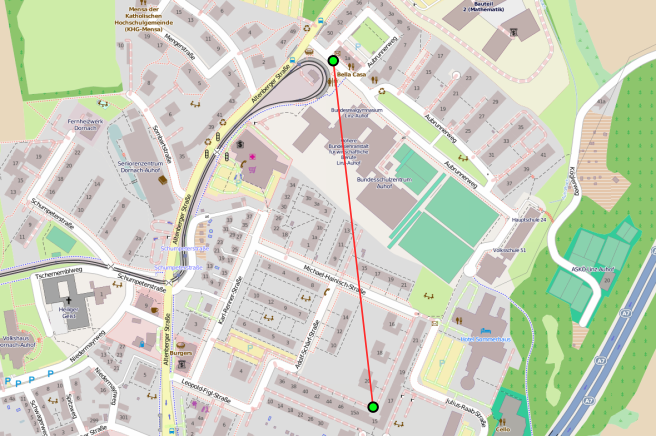
          This is of course the easiest way: all data about the map is ignored. This strategy makes sense if you need a geo-spatial coordinate system, but you are simulating objects that are mostly or entirely unaffected by the street-level structure (buildings, roads, etc.); for instance, if the simulation involves unmanned aerial vehicles. There is no need of importing actual map data when navigating this way.

          This kind of navigation can be realized using MoveToTarget.

          Examples

          Click to show / hide code
          Click to show / hide code

          From the showcase

          Optimal resilient distributed data collection in mobile edge environments

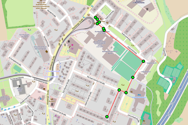
          navigate along the streets navigate along the streets

          Moves along the available paths, depending on the specific vehicle being used. Requires actual geo-spatial information.

          This kind of navigation can be realized using TargetMapWalker.

          Reproduce a GPS Trace

          reproduce a GPS trace reproduce a GPS trace

          Ignores the map geospatial information and relies on a GPS trace instead, starting from its first position and reaching the last, navigating from point to point in “straight lines” (on maps, these are actually orthodromes).

          This kind of navigation can be realized using ReproduceGPSTrace.

          Deploying nodes using GPS traces

          You probably want your nodes to start from the position that marks the beggining of a trace. We discussed how to do so here.

          Time alignment of GPS traces

          Navigation with GPS traces usually require that they get correctly aligned with time, especially if they come from samples taken at different times. We discussed the alignment of GPS traces here, the same alignment system used for importing traces is used for using them during navigation.

          Examples

          Click to show / hide code

          Interpolate GPS traces with street data

          interpolate GPS traces interpolate GPS traces

          Navigates along a GPS trace, but computes the point-to-point distance using the navigation system, rather than “straight lines” (orthodromes).

          This kind of navigation can be realized using GPSTraceWalker.

          Node contents

          It is possible to set the content of the nodes in a deployment. Node contents are defined in terms of molecules and their corresponding concentration. As such, they depend on the specific Incarnation in use.

          This is done by listing the contents under deployments.contents, specifying a Molecule name and its Concentration.

          Unless the type/parameter syntax is used, the data gets processed by the Incarnation through the Incarnation.createMolecule and Incarnation.createConcentration methods, respectively.

          In the following example, three molecules are created and injected into all nodes deployed in the scenario:

          Click to show / hide code

          By default, all nodes in the deployment will be injected with the required contents. It is possible, though, to select only a subset of them through the in keyword, which expects enough information to be able to build a PositionBasedFilter through the arbitrary class loading system.

          In the following example, only molecules located inside a Rectangle get the ball molecule:

          Click to show / hide code

          Smart cameras and drones

          <div style="position: relative; padding-bottom: 56.25%; height: 0; overflow: hidden;">
            <iframe allow="accelerometer; autoplay; clipboard-write; encrypted-media; gyroscope; picture-in-picture; web-share" allowfullscreen="allowfullscreen" loading="eager" referrerpolicy="strict-origin-when-cross-origin" src="https://www.youtube.com/embed/yuaY_8Vr3oc?autoplay=0&amp;controls=1&amp;end=0&amp;loop=0&amp;mute=0&amp;start=0" style="position: absolute; top: 0; left: 0; width: 100%; height: 100%; border:0;" title="YouTube video"></iframe>
          </div>
          

          Prerequisites

          This guide assumes you already know the Alchemist metamodel and that you keep the YAML reference at your fingertips.

          Smartcam

          A smartcam is a camera able to detect objects of interest and to communicate with other smartcameras. In many cases it is also assumed to be mounted on a drone as to be able to freely move around in the environment. In Alchemist, smartcams are simulated as Nodes equipped with specific Reactions defining their capabilities and behaviour. Single capabilities are expressed as Actions.

          Vision

          The most basic example of a camera is a Node containing a Reaction with the CameraSee action.

          Warning

          Note: the CameraSee action currently only works in 2D environments supporting euclidean geometry, for example Continuous2DEnvironment.

          CameraSee requires the following parameters:

          1. the distance of the field of view,
          2. its angle in degrees, and
          3. the name of the Molecule which will contain the ouput, namely, the list of nodes contained in the field of view, which is updated every time the action is triggered,
          4. optionally, a fourth parameter can be defined in order to filter the output, such parameter is expected to be the name of a Molecule which has to be contained in a Node for it to be visible, e.g., if it is wanted then only nodes containing a molecule named wanted will be seen.

          Movement

          The ability to move can be defined using movement actions such as MoveToTarget or FollowAtDistance.

          MoveToTarget expects 2 parameters:

          1. the name of the molecule containing the target’s position, and
          2. the movement speed.

          FollowAtDistance requires:

          1. the name of the molecule containing the target’s position,
          2. the distance to mantain from the target, and
          3. the movement speed.

          Rotation

          HeadTowardTarget can be used to instruct cameras to always face the specified target.

          Spin only requires the angular speed and will make the camera spin around itself like a radar.

          Other behavior

          Without defining an algorithm the cameras wouldn’t do anything interesting. Algorithms can be definied in a moltitude of different ways, depending on the incarnation. Usually, camera readings are used as sensors that get read by, e.g., Protelis or Scafi programs.

          Further references

          Lukas Esterle, Peter R. Lewis
          Online Multi-object k-coverage with Mobile Smart Cameras
          In Proceedings of the International Conference on Distributed Smart Cameras (ICDSC). Nominated for best paper. 2017.

          Subsections of Execution

          Customize the Swing GUI

          T.B.D.

          Drawing navigation graphs

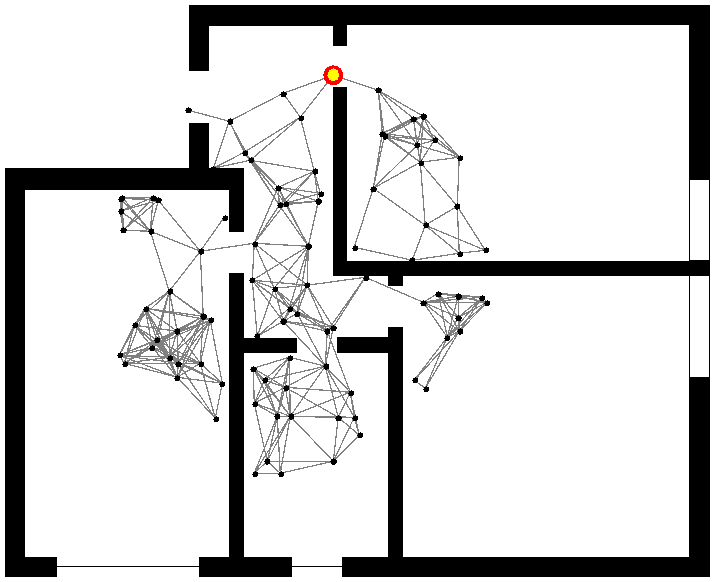
          The GUI includes a simple effect to draw the navigation graph of an ImageEnvironmentWithGraph in the gui is available as well. Its name is DrawNavigationGraph, you can just select it from the available effects in the gui to have your graph drawn.

          Define the termination criteria

          Alchemist supports the possibility to write termination conditions for any simulation. Termination conditions are checked after every event, and, if met, cause the immediate termination of a simulation. Termination conditions are expected to be found in the {{ anchor(‘it.unibo.alchemist.model.implementations.terminators’) }} package.

          They are defined in the terminate section of the configuration file. Multiple terminators are allowed, the first terminator matching causes the termination of the simulation (they are in and).

          Terminating the simulation after some time

          One of the simplest terminators availables allows for declaring a simulation completed when a certain simulated time is reached. In the following example, it is used in conjunction with a number of variables, showing how it’s possible to use such variables to produce batches of simulations terminating at different times.

          Click to show / hide code

          Terminating the simulation if the environment is not changing

          A terminator is provided for terminating when a simulation is “stable” (nothing changes in terms of positions and nodes’ content). The class implementing it is StableForSteps.

          MultiVeStA

          Once you have your simulation project configured as you want, you need to:

          1. Add dependency on the multivesta jar implementation(files("libs/multivesta.jar")). You can require the jar by going to MultiVesta’s repository
          2. Include the following dependency in build.gradle.kts implementation("it.unibo.alchemist:alchemist-multivesta-adapter")
          3. Copy the AlchemistSimState class from current repo (you can reach it in following location alchemist-multivesta-adapter/dist/AlchemistSimState.kt) and paste it in the package you prefer
          4. Set the main class as follows mainClass.set("it.unibo.alchemist.multivesta.adapter.AlchemistMultiVesta"), inside the JavaExec Gradle task
          5. When you configure Alchemist arguments with Gradle args method, add another args call after traditional Alchemist arguments and pass all MultiVeStA arguments in a single string with key "-mv", e.g. args("-mv", "-c -sots 1 -bs 30 -a 0.05 -ds [0.1] -l 12 com.example.AlchemistSimState -f myquery.multiquatex").
            Important: MultiVeStA arguments must include the fully qualified name of the class you have copied on point 3 (in the example it is -com.example.AlchemistSimState) and the desired multiquatex file (in the example it is -f myquery.multiquatex)
          6. Add MultiVestaExporter to your Alchemist configuration file, specifying the desired Extractor type: it will supply all available properties to MultiVeStA

          If you prefer avoiding to add the exporter in Alchemist configuration file, you can add the Alchemist argument -e ExporterClass, that will use such exporter to supply the desired observation to MultiVeStA.

          You are now ready to start your simulation as usually with Gradle JavaExec task!

          Parameter Sweeping with simulation batches

          In some cases you may need to test the same simulation configuration with different parameters. Suppose for example that you want to see what happens when you place a bunch of pedestrian in a circle (for sake of semplicity we’ll ignore their behavior). You may want to observe the scenario with 50 pedestrians placed in a 5 meters radius circle. Then you may like to observe it with 100 pedestrian and perhaps by changing the circle radius also. Instead of re-writing the configuration file over-and-over for each parameter combination, Alchemist offers the possibility to write the configuration once, and it will then derive a batch of simulations.the same configuration

          Launching batch simulations

          To exploit this mechanism, you must declare the “parameters” as variables. In our example, they would be the number of pedestrian and the radius of the circle where to place them. Let’s write the configuration file, specifing that we want to test the simulation with 10, 30, 50, 70, 90 pedestrians and a 5, 10, 15 meters circle radius:

          Click to show / hide code
          Info

          To understand how variables work refer to this page. You may also want to learn how to export data and specifying termination criteria.

          Now we can launch the batch of simulations by providing the simulator the following command-line arguments:

          • -b: enable batch mode
          • -var pedestrianNumber: all values of variable pedestrianNumber will be tested
          • -var circleRadius: all values of variable circleRadius will be tested

          Under the hood, the simulator will compute the cartesian product of the all possible values of the variables selected with the -var option. Variables not selected for the batch will have their default value.

          Simulation Engine Configuration

          Engine Configuration

          The default Alchemist execution requires no special configuration, however different engine implementations are available.

          In order to configure a different engine, simply add an EngineConfiguration object into the simulation configuration file as per the alchemist Arbitrary class loading system.

          Parallel Batch Engines

          Parallel batch engine is an implementaion of Alchemist’s base engine that speeds up the computations by processing event batches in parallel at the price of determinism.

          All batch engine implementations require the following parameters:

          • outputReplayStrategy - determines how the output monitors get notified after the batch has been processed. Available values:
            • aggregate - only the state after the batch processing is sent to the monitors
            • replay - all the state changes get sent to the monitors ordered by scheduled time.

          Fixed Size Batch Engine

          Fixed size batch engine processes events in parallel in batches of fixed size.

          Sample configuration:

          engine-configuration:
            type: FixedBatchEngineConfiguration
            parameters:
              outputReplayStrategy: aggregate
              batchSize: 4

          Epsilon Batch Engine

          Epsilon dynamic size batch engine processes events in parallel in batches constructed using the epsilon sensitivity value. Events get added to the batch as long as the difference in scheduled time is lesser than the given epsilon value.

          Sample configuration:

          engine-configuration:
            type: EpsilonBatchEngineConfiguration
            parameters:
              outputReplayStrategy: aggregate
              epsilonValue: 0.01

          0.01 is a reasonable baseline, experiment to find the best value for your case.

          Workarounds

          Pre-concocted solutions to well-known issues

          Work arounds

          If your problem is not listed here, it may still be known and a discussion/workaround could be available on the Alchemist Github issue tracker.

          Other issues you may experience are listed below.

          Warning

          Contents

          Subsections of Workarounds

          Graphical Glitches in Swing

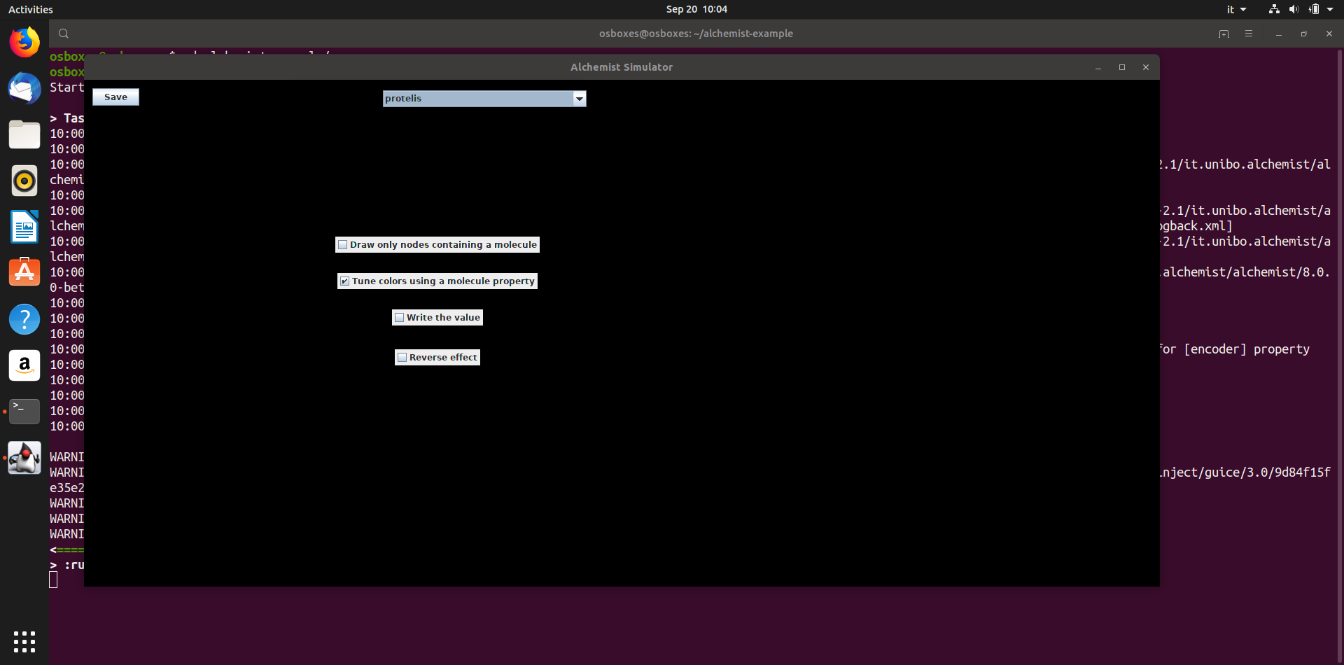
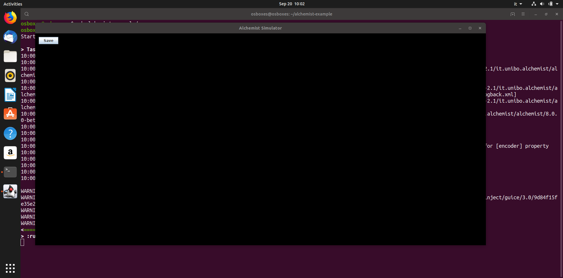
          Under some combination of hardware and drivers, the Swing interface may render uncorrectly. This is due to Alchemist using OpenGL as rendering backend for Swing, in order to increase performance.

          Examples of graphical glitches, on a VirtualBox instance with Ubuntu

          Graphical glitch example Graphical glitch example Graphical glitch example Graphical glitch example Graphical glitch example Graphical glitch example

          Solution

          Disable the OpenGL acceleration explicitly by setting the sun.java2d.opengl property to false.

          Gradle

          With Gradle, edit the Alchemist launch task (which should be a JavaExec) by adding: jvmArgs("-Dsun.java2d.opengl=false")

          Stand-alone

          Add the appropriate JVM option:

          java -Dsun.java2d.opengl=false -jar alchemist-full.jar

          Memory leaks under Linux

          When Alchemist is used on computers with a large amount of memory and parallelism, additional configuration might be required.

          Info

          These problems have more to do with the way memory allocation on Linux and the JVM works than with Alchemist itself. They are not memory leaks in Alchemist (hence the reason why they do not happen with smaller memory sizes).

          Symptoms

          • batch execution slowing down (this is due to the memory pressure)
          • analysis of memory shows that the amount of memory actually in use by the JVM is always growing (similar to a memory leak)
          • the following (or similar) warning is displayed on the standard error on startup:
          [warning][gc] ***** WARNING! INCORRECT SYSTEM CONFIGURATION DETECTED! *****
          [warning][gc] The system limit on number of memory mappings per process might be too low for the given
          [warning][gc] max Java heap size (101754M). Please adjust /proc/sys/vm/max_map_count to allow for at
          [warning][gc] least 183157 mappings (current limit is 65530). Continuing execution with the current
          [warning][gc] limit could lead to a premature OutOfMemoryError being thrown, due to failure to map memory.

          Solution

          Warning

          The file /proc/sys/vm/max_map_count could be changed manually, but these changes won’t persist reboots.

          A persistent solution to the problem is to instruct the system to always load the correct configuration. One possible way is to instruct sysctl through a configuration file (e.g., /etc/sysctl.d/99-vm-max-map-count.conf) including the following line: vm.max_map_count=<custom max_map_count>. This can be done on a root shell via:

          sudo sh -c 'echo "vm.max_map_count=<custom max_map_count>" > /etc/sysctl.d/99-vm-max-map-count.conf'
          sudo sysctl --system
          Computing a “good” value for max_map_count

          A reasonable estimation of the value is four times the amount of system RAM expressed in Megabytes (for instance vm.max_map_count=524288 for a system with 128GB RAM).

          When in doubt, select a higher value, apparently the negative effects are negligible.

          Ready-to-use commands

          • 128GB
          sudo bash -c 'echo "vm.max_map_count=524288" > /etc/sysctl.d/99-vm-max-map-count.conf' && sudo sysctl --system
          • 256GB
          sudo bash -c 'echo "vm.max_map_count=1048576" > /etc/sysctl.d/99-vm-max-map-count.conf' && sudo sysctl --system
          • 512GB
          sudo bash -c 'echo "vm.max_map_count=2097152" > /etc/sysctl.d/99-vm-max-map-count.conf' && sudo sysctl --system
          • 1TB
          sudo bash -c 'echo "vm.max_map_count=4194304" > /etc/sysctl.d/99-vm-max-map-count.conf' && sudo sysctl --system

          Experiment-specific extensions

          One-time changes or additions to the simulator behavior

          Experiment-specific extensions

          Contents

          Subsections of Development

          Developer's guide

          Contributions to this project are welcome. Just some notes:

          • Use conventional commits. The build auto-generates aggressive git hooks that enforce the rules.
          • Contributions must be realized in forks of the project. Once a contribution is ready, please open a pull request.
          • Keep in sync with the mainline (our master branch), preferably via rebasing.
          • Commit often. Small pull requests targeting a small part of a larger work are very welcome if they can be merged individually.
          • Do not introduce low quality code. All the new code must comply with the checker rules (that are quite strict) and must not introduce any other warning. Resolutions of existing warnings (if any is present) are very welcome instead.
          • Fixes should include a regression test.
          • New features must include appropriate test cases.
          • Any change should cause an extension or modification of the documentation, that must be kept up to date

          Enrich the GraphQL API

          It is possible to integrate new queries, mutations, or subscriptions into the GraphQL API. This augmentation offers a more organized and predictable approach for interacting with the simulator, thanks to static typing and schema definition.

          It is possible to use GraphQL APIs for the development of a module inside Alchemist. The GraphQLClient class will take care of establishing a connection to the GraphQL server, validate and compute operations and return their results. This component has been developed in a multiplatform environment, so that applications can run on platforms like Android, iOS, Kotlin/JS or Kotlin/Native.

          Create a new Query, Mutation, or Subscription

          In order to create new queries, mutations, or subscriptions, follow these steps:

          1. Include the alchemist-graphql common source set in your project.
          implementation(alchemist("graphql"))
          1. Define the structure of the data you need when executing one of the provided operations, inside a set of files with .graphql extension placed in the alchemist-graphql/src/commonMain/resources/graphql/ directory. The following is an example of a query that retrieves the contents of a node by its ID:
          # NodeQuery.graphql
          query Node($id: Int!) {
              nodeById(id: $id) {
                  contents {
                      entries {
                          molecule {
                              name
                          }
                          concentration
                      }
                  }
              }
          }
          Use GraphiQL to build client’s operations files

          You can test the structure of the data that you need inside the GraphiQL playground, in order to get predicable results when compiling your operations. GraphiQL also notices you if you are writing incorrect operations with useful explanation about the errors.

          1. Run the Gradle task ./gradlew :alchemist-graphql:generateApolloSources in order to generate Kotlin’s source code that represents the results of operations called in previously defined files.

          2. Use the defined GraphQL compiled operations on top of the GraphQLClient to execute them.

          val client: GraphQLClient = GraphQLClientFactory.basicClient()
          /* `NodeQuery` is the generated code for the
              GraphQL operation defined in the example above */
          val node: Node? = client.query(NodeQuery(nodeId = 10)).execute().data

          Import Alchemist in an IDE

          The project is easiest to import in IntelliJ Idea. The project can be imported directly as a Gradle project. If you intend to develop new parts in Scala, we suggest to install the Scala plugin for IntelliJ Idea.

          Forking the project

          To contribute to the Alchemist project you must fork it and work on your own copy. In this way you can:

          • push all your commits, saving your work on the cloud;
          • exploit the included continuous integration jobs to check the project status;
          • contribute back to the main project via pull requests directly from GitHub.

          Importing the project

          1. Clone either the Alchemist repository or your personal fork in a folder of your preference using git clone --recurse-submodules <ALCHEMIST_REPO_URI>.
          2. Right click on settings.gradle.kts, select “Open With” and use IntelliJ Idea.

          The procedure may be slightly different depending on your operating system and desktop environment.

          If you have a terminal, and if you can launch idea from there, just:

          1. cd <LOCATION_WHERE_YOU_CLONED_THE REPOSITORY>
          2. idea . (we are assuming that you can launch IntelliJ Idea with the idea command, replace it with the correct one for your system)

          Build and run the QA

          Building with Gradle

          The recommended way to execute any Gradle build is with the help of the Gradle Wrapper (in short just “Wrapper”). The Wrapper is a script that invokes a declared version of Gradle, downloading it beforehand if necessary. As a result, developers can get up and running with a Gradle project quickly without having to follow manual installation. For more information please refer to the Gradle’s documentation website.

          gradlew vs. gradlew.bat

          Depending on which scripting environment you are using the wrapper can be invoked with gradlew or gradlew.bat. Windows users are likely to use the latter.

          Building the project

          The project can get build via Gradle:

          ./gradlew assemble --parallel

          When imported in IntelliJ Idea as Gradle project, the IDE will use Gradle under the hood to run the necessary steps to perform compilation and packaging.

          Testing

          Testing can be executed by issuing

          ./gradlew test --parallel

          Quality Assurance

          To perform a QA run

          ./gradlew check --parallel

          Generating the website

          To generate the Alchemist website run

          ./gradlew hugoBuild --parallel

          Website preview

          For a preview of the website issue:

          ./gradlew hugo --command=serve

          The terminal output will show a link, most likely https://localhost:1313/, where the website is being served.

          Explanation

          Understanding-oriented

          Explanation

          Contents

          Subsections of Explanation

          The Alchemist Meta-Model

          The first step to take in order to use the simulator, is to answer the question

          what does Alchemist simulate?

          A broad introduction is provided in form of introductory video from the DAIS 2021 conference tutorial.

          The model

          The world of Alchemist is composed of the following entities:

          • Molecule
            • The name of a data item
            • If Alchemist were an imperative programming language, a molecule would be the concept of variable name
          • Concentration
            • The value associated to a particular molecule
            • If Alchemist were an imperative programming language, a concentration would be the concept of value associated to a variable
          • Node
            • A container of molecules and reactions, living inside an environment
          • Environment
            • The Alchemist abstration for the space. It is a container for nodes, and it is able to tell:
              1. Where the nodes are in the space - i.e. their position
              2. The distance between two nodes
              3. Optionally, support for moving nodes
          • Linking rule
            • A function of the current status of the environment that associates to each node a neighborhood
          • Neighborhood
            • An entity composed by a node (centre) and a set of nodes (neighbors)
          • Reaction
            • Any event that can change the status of the {{ anchor(’environment’, ‘Environment’) }}
            • Each node has a possibly empty set of reactions
            • Each reaction is defined by a possibly empty list of conditions, one or more actions and a {{ anchor(’time distribution’, ‘TimeDistribution’) }}
            • The frequency at which it happens depends on:
              1. A static “rate” parameter
              2. The value of each condition
              3. A “rate equation”, that combines the static rate and the value of conditions, giving back an “instantaneous rate”
              4. A time distribution
          • Condition
            • A function that takes the current environment as input and outputs a boolean and a number
            • If the condition does not hold (i.e. its current output is false), the reaction to which it is associated cannot run
            • The outputed number may or may not influence the reaction speed (i.e. the average number of times the reaction “happens” per time unit), depending on the reaction and its time distribution.
          • Action
            • Models a change in the environment.

          The following image is a visualization of such model:

          Alchemist model Alchemist model

          The behavior of the system is described in terms of reactions. As such, here’s a pictorial representation of a reaction:

          Alchemist reaction Alchemist reaction

          Incarnations

          As you can see, names are given after classical chemistry terms. This is mostly for historical reasons: Alchemist has been initially conceived as a chemical-oriented multi-compartment stochastic simulation engine, able to support compartment (node) mobility while still retaining high performance.

          However, Alchemist is not limited to that. The key of its extensibility is in the very loose interpretation of molecule and concentration. These two terms have a very precise definition in chemistry, but in Alchemist they are respectively

          1. a generic identifier, and
          2. a piece of data of some type

          An incarnation of Alchemist includes a type definition of concentration, and possibly a set of specific conditions, actions and (rarely) environments and reactions that operate on such types. In other words, an incarnation is a concrete instance of the Alchemist meta-model. In addition, a proper Alchemist incarnation’, ‘Incarnation must also define:

          • Means for translating strings into named entities (molecules)
          • Means for obtaining a number when given a node, a molecule and a string representing a property
          • Means for building incarnation-specific model entities given an appropriate context and a parameter String

          These functionalities are required in order to support a uniform access to different incarnations.

          Different Incarnations can model completely different universes. For instance, if the concentration is defined as a positive integer and proper actions and conditions are provided, Alchemist becomes a stochastic simulator for chemistry featuring interconnected and mobile compartments.

          The standalone distribution comes with:

          The Alchemist Simulation Engine

          The core part of the tool is the incarnation-agnostic simulation engine. Its current implementation is based on Gibson and Bruck’s Next Reaction, extended to support addition and removal of reactions, and improved using input and output contexts for reactions, in order to prune the dependency graph as much as possible. More details on that are demanded to this scientific paper on Journal of Simulation.

          The engine’s entry point is the Simulation. It is equipped with support for commands like play, pause and stop, and can be equipped with an OutputMonitor. The output monitor can be a graphical interface, a logger or any kind of environment inspector.

          Biochemistry Incarnation

          Biochemistry is an incarnation of Alchemist developed to provide support for biochemical reactions that take place inside a biological cell or a group of those surrounded by a common environment.

          The Biochemistry Incarnation

          The Biochemistry incarnation provides ways to:

          • Manage the creation, destruction and relocation of a molecule (which can be either a simple atom or a complex protein) inside a cell or from a cell to another
          • Create junctions between cells using a specified amount of molecules. The junctions are modeled in a general way, but with a simple use of actions and conditions it will be possible to create tight junctions, anchoring junctions, gap junctions and even custom one
          • Move a cell inside its environment in different ways, handling collisions between two ore more of them in a simple but effective way

          The Biochemistry DSL

          Biochemistry programs are encapsulated inside the YAML configuration file with a simple and human-readable syntax. Those simple reactions can be written in the section programs of the configuration file, as value of the program key:

          programs:
            -
              - time-distribution: 1
                program: "[ATP] --> [ADP] + [P]"

          Reactions

          A reaction rule can be set using the symbol --> according to chemistry equations, and placing both the molecules and the actions inside two square brackets (ex. [OH], [H2O], [BrownianMove(0.1)])

          The following line, so, represents a basic chemical reaction that happens inside a cell: [H] + [OH] --> [H2O]

          However, reactions can also take place outside the cell itself. Biological cells, indeed, can swap molecules with its neighbour or the surrounding environment, and this is possible in Alchemist too, using the keywords: in cell, in neighbour and in env.

          The reaction [A in env] --> [A in cell] moves the molecule A from the environement inside the cell.

          If the location is not explicit, it is assumed the molecule to be inside the cell.

          Junctions

          A junction can be created just with a neighbor of the programmed cell.

          The way to create it is with the syntax [X] + [Y in neighbor] --> [junction X-Y], which means that when this reaction happens a junction using the molecule X from the cell and the molecule Y from the neighbor will be created.

          The junction can also be destroyed using the syntax [junction X-Y] --> [], causing the reintroduction of the molecule X inside the cell and the molecule Y inside the neighbor.

          Also, the junction will be automatically removed if, because of their movement, the cells will stop being in a neighborhood.

          Custom Conditions

          Any custom condition must be placed after the reaction products following an if clause.

          For example, to create a molecule if the cell has at least three neighbor you would write:

          [] --> [X] if NumberOfNeighborsGreaterThan(5)

          Movement

          A movement can be performed in the same way of a reaction, using the function as it is a product of the reaction itself.

          This program constantly moves a cell without any other condition:

          [] --> [BrownianMove(0.1)]

          Collisions

          The Biochemistry Incarnation supports cell collisions and deformations too.

          In order to do that, however, you must set this environment:

          environment:
            type: BioRect2DEnvironmentNoOverlap

          Then, when creating the cells, you must use these specific implementations:

          nodes:
            type: CircularDeformableCellImpl
            parameters: [max-radius, rigidity]

          The minimum radius of the cell is so that min-radius = rigidity * max-radius and the two parameters are used to compute collisions and impacts between the cells.

          Cognitive Agents

          Alchemist is capable of simulating the movement of pedestrians with sophisticated cognitive capabilities:

          demo demo

          The animation above shows an adult male with no previous knowledge of the environment trying to reach the destination marked green.

          Types of pedestrian

          There are three basic types of pedestrian, each representing a more sophisticated version of the previous one. These are derived from the work of van der Wal et al.

          1. Homogeneous Pedestrians: Nodes with no peculiar characteristic.
          2. Heterogeneous pedestrians have an age and a gender, based on which their speed, compliance to rules, and social attitudes are computed.
          3. Cognitive pedestrians are heterogeneous pedestrians with cognitive capabilities. They have an emotional state and are able to influence and be influenced by others with the same capabilities. As an example, cognitive pedestrians can perceive fear via social contagion (e.g. seeing other people fleeing may cause them flee as well regardless of whether they’ve seen the danger directly).
          4. Orienting pedestrians, as shown in the animation on the top of the page, can be equipped with different knowledge degrees of the environment. To do so, a particular type of pedestrian called orienting pedestrian is required: this is derived from the work of Andresen et al.

          Types of behaviors

          There are two macro-categories of behaviours:

          • those inspired to Reynold’s steering behaviors, which operate in a greedy fashion, i.e. performing only local choices;
          • those inspired to the work of Andresen et al, which exploit the spatial information available to orienting pedestrians in order to navigate the environment consciously (e.g. without getting stuck in U-shaped obstacles). Note that these actions do not assume that pedestrians have global knowledge of the environment, on the contrary only the spatial information available to a pedestrian is used to move it (which can be little or nothing).

          Each time a pedestrian enters a new room (= environment’s area), all the visible doors are weighted, the one with minimum weight is then crossed. The weighting system used in Alchemist is derived from the one by Andresen et al, here’s a brief description of the factors included, these are multiplied to get the final weight.

          Name Description
          volatileMemoryFactor Takes into account the information stored in the pedestrian’s volatile memory (= a map pairing each room with the number of visits, models the ability to remember areas of the environment already visited since the start of the simulation). It is computed as 2^v where v is the number of visits to the area the edge being weighted leads to (in other words, less visited rooms are preferred).
          congestionFactor Takes into account the congestion of the area the edge being weighted leads to (it is assumed that the pedestrian can estimate the congestion level of a neighboring room). It is computed as density of the area + 1, so as to have a value in [1,2] (less crowded rooms are preferred).
          impasseFactor Takes into account whereas a door leads to a known impasse or not, known impasses are given knownImpasseWeight (see hardcoded parameters below), otherwise this factor assumes unitary value.
          suitabilityFactor This factor is used when the pedestrian is moving towards a target: each door is given an integer rank indicating its suitability in order to reach the target (ranks are computed taking into account the target and the door locations, as well as the geometry of the current room). The factor for each door is computed as 1-0.5^rank.

          Physical pedestrians

          Physical pedestrians are capable of pushing and bumping into each other. Physical pedestrians are inspired to the work of Pelechano et al.

          Further references

          C. Natalie van der Wal, Daniel Formolo, Mark A. Robinson, Michael Minkov, Tibor Bosse
          Simulating Crowd Evacuation with Socio-Cultural, Cognitive, and Emotional Elements
          Transactions on Computational Collective Intelligence XXVII. 2017.

          Craig W. Reynolds
          Steering Behaviors for Autonomous Characters. 1999.

          Erik Andresen, Mohcine Chraibi & Armin Seyfried
          A representation of partial spatial knowledge: a cognitive map approach for evacuation simulations

          Nuria Pelechano, Jan M. Allbeck, Norman I. Badler
          Controlling Individual Agents in High-Density Crowd Simulation

          Pathfinding

          This section explains the pathfinding strategies and algorithms of Alchemist. Instructions on how to exercise them are available here.

          A navigation graph of an environment with obstacles is a graph whose nodes are convex shapes representing portions of the environment which are traversable by agents (namely, walkable areas), and edges represent connections between them. The image below shows a bidimensional environment with obstacles on the left and the associated navigation graph on the right (nodes are painted blue, edges are represented as line segments connecting the centroid of a node to the associated crossing, which is painted green).

          navigation graph navigation graph

          Navigation graphs are mainly used for navigation purposes (e.g. in pathfinding algorithms): the advantage of decomposing the environment into convex regions is that agents can freely walk around within a convex region, as it is guaranteed that no obstacle will be found (remember that a shape is convex when no line segment between any two points on its boundary ever goes outside the shape).

          Alchemist is capable of generating navigation graphs of bidimensional environments featuring euclidean geometry and double precision coordinates. Before diving into the topic, please be aware that the algorithm implemented in Alchemist for the generation of navigation graphs:

          • Does not guarantee the coverage of 100% of the walkable area (as the image above shows).
          • Is only capable to detect axis-aligned crossings.
          • Is only capable to deal with convex polygonal obstacles. Concave ones can be decomposed into convex meshes, whereas for curves bounding boxes can be used, eventually arbitrarily-oriented minimum bounding boxes.

          The algorithm implemented in Alchemist is called NaviGator (Navigation Graphs generAtor), here’s a brief description of how it operates: firstly, a certain number of seeds is planted in the environment. Each seed is a square-shaped region of unitary side that will grow maintaining a convex shape. Secondly, planted seeds are extended as far as possible (i.e. until they are in contact with an obstacle or another seed on each side). Finally, crossings are found between the grown seeds. NaviGator is derived from the DEACCON algorithm for the generation of navigation meshes.

          SAPERE Incarnation

          The SAPERE incarnation for Alchemist was the first stable incarnation produced for the simulator. It was developed in the context of the SAPERE EU project.

          At the core of SAPERE is the concept of Live Semantic Annotation (LSA), namely a description of a resource (sensor, service, actuator…) always mapping the current resource status (somewhat a prelude to the currently famous digital twin concept).

          These annotations evolve following so-called Eco-Laws, mimicking the complex behaviours of natural ecosystems.

          The SAPERE approach fostered subsequent approaches, such as aggregate computing.

          Live Semantic Annotations

          An LSA as modeled in Alchemist is a tuple of values. These tuples can be injected in nodes as data items. From the point of view of the Alchemist metamodel, the concept of Molecule is mapped to LSA (LsaMolecule). As a consequence, LSAs can be inserted in nodes.

          Eco-Laws

          Tuple matching is used to define Eco-Laws. An Eco-Law is a rewriting rule very similar in concept to chemical reactions: elements on the left-hand side of the reaction are removed from the container, elements on the right-hand side are inserted instead.

          The following program matches LSAs with two arguments, the former must be foo, the latter a number greater than 30, and produces in a new tuple having as first element bar and as second the opposite of the matched number:

          { foo, def: N > 30 } --> { bar, -N }

          Reference

          Information-oriented

          Reference

          Contents

          Subsections of Reference

          YAML simulation specification

          Warning

          This reference guide assumes that the reader knows the basics of YAML. A good resource to learn it quickly is Learn X in Y minutes where X = YAML

          Reading this document

          The key words MUST, MUST NOT, REQUIRED, SHALL, SHALL NOT, SHOULD, SHOULD NOT, RECOMMENDED, MAY, and OPTIONAL in this document are to be interpreted as described in RFC 2119.

          Simulation document structure

          The document MUST be YAML map. The map MUST contain all the mandatory Alchemist keys, MAY contain any subset of the optional Alchemist keys, MAY contain any key whose name begins with underscore (_), and MUST NOT contain any other key.

          The sets of valid cobinations of mandatory and optional keys for each section of the document is specified in form of Kotlin code as follows:

          Types of entries

          Type Description
          Any Any YAML type
          Int YAML integer number, or other type that can be parsed into an integer
          List Any YAML List
          Map Any YAML Map
          MultiSpec A list of Spec. A Map matches a MultiSpec if it matches one and only one of its Spec.
          Number YAML number
          Spec Pair of lists of strings. The first list contains mandatory keys, the second optional keys. A map matches a Spec if it contains all its mandatory keys, any of the optional keys, and no other key
          SpecMap A YAML Map matching a MultiSpec
          String YAML String
          Traversable One of: A SpecMap, a List of Traversable, a Map of Traversable

          Arbitrary class loading system

          Type: SpecMap

          Alchemist is able to load arbitrary types conforming to the expected interface (or Scala trait). The expected type depends on where the class is requested. This section describes how the system works independently of the specific target type.

          (Multi)Spec

          Mandatory keys Optional keys
          type parameters

          type

          Type: String

          The name of an instanceable class compatible with the expected interface. It can be either the qualified name or a simple name, in the latter case the class SHOULD be located in the same package where the default alchemist implementations of the same interface live.

          If a name includes a ., it is interpreted as a fully qualified name. Otherwise, it is interpreted as a simple name. Provided types SHOULD NOT be located in the default package.

          For instance, if the expected type is an Action and the concrete type FooAction, FooAction SHOULD be located into package it.unibo.alchemist.model.actions.

          parameters

          Type: List or Map

          The list of parameters the constructor of type should be passed. Alchemist automatically provides contextual information to the constructors: for instance, if an Action is being built, the loading system is aware of the current RandomGenerator, Incarnation, Environment, Deployment, Node, TimeDistribution, and Reaction, as the action requires all of them. Consequently, all parameters of these types SHOULD NOT be manually specified (on the other hand, the syntax is built to make it very difficult to do by mistake). The constructor MAY fail if they are provided.

          If a Map is provided instead of a List, then the keys are interpred as the parameter names, and their associated values as the corresponding parameter values. Since Java 11 does not support named arguments, this special invocation type is built around the Kotlin reflection, thus, the concrete class whose constructor is being invoked MUST be written in Kotlin.

          When using named arguments, if at least one optional parameter is specified, then all the previous optional parameters MUST be specified as well. This limitation is due to the fact that Alchemist supports loading of JVM classes regardless of their origin language, and, thus, the simulator must leverage constructor overloading to emulate optional parameters. In the case of Kotlin classes, because of the way @JvmOverloads works, only a (reasonable) subset of all possible overloads gets generated, and they differ by parameter count.

          Instantiation is delegated to the Java Implicit Reflective Factory.

          Examples

          • Construction of a Point
            Click to show / hide code
          • Construction of variables with named parameters
            Click to show / hide code

          Counter-examples

          • The following simulation fails on loading, as BidimensionalGaussianLayer has the first and last parameters marked as optional: in order to provide the latter, the designer must also provide the former.
            Click to show / hide code

          Document root

          Type: SpecMap

          The document contents at the root of the file. Contains all the information required to buld a Loader, which, in turn, is able to spawn Simulations through a Launcher.

          (Multi)Spec

          Mandatory keys Optional keys
          incarnation deployments, environment, export, layers, launcher, network-model, remote-dependencies, seeds, terminate, variables

          Examples

          • Minimal Biochemistry specification
            Click to show / hide code
          • Minimal Protelis specification
            Click to show / hide code
          • Minimal SAPERE specification
            Click to show / hide code

          incarnation

          Type: String

          Valid incarnation types in the full distribution:

          • biochemistry
          • protelis
          • sapere
          • scafi

          Examples

          • Minimal Biochemistry specification
            Click to show / hide code
          • Minimal Protelis specification
            Click to show / hide code
          • Minimal SAPERE specification
            Click to show / hide code

          action

          Builds an Action using the arbitrary class loading system.


          condition

          Builds a Condition using the arbitrary class loading system.


          deployments

          Type: Traversable

          Traversable of deployment

          deployment

          Type: SpecMap

          Definition of the positions of a set of nodes. Builds a Deployment using the same syntax of arbitrary class loading system, with additional keys.

          (Multi)Spec

          Mandatory keys Optional keys
          type parameters, contents, nodes, programs

          Examples

          • Deployment of a single node in a point
            Click to show / hide code
          • Deployment of three nodes
            Click to show / hide code
          • Deployment of three nodes, but nesting the traversable
            Click to show / hide code
          • Deployment of three nodes through SpecificPositions.
            Click to show / hide code
          • Grid centered in (0, 0), with nodes distanced of 0.25 both horizontally and vertically.
            Click to show / hide code
          • Irregular Grid centered in (0, 0), with nodes distanced of 0.25 both horizontally and vertically, randomly perturbed of (±0.1 distance units).
            Click to show / hide code
          • Nodes located randomly inside a Circle
            Click to show / hide code
          • Nodes located randomly inside a Rectangle
            Click to show / hide code
          • Nodes located randomly inside a Polygon delimiting the Venice Lagoon
            Click to show / hide code

          deployment.type

          Same as type

          deployment.parameters

          Same as parameters

          deployment.contents

          Type: Traversable of content

          deployment.nodes

          Type: SpecMap

          Forces the type of Node, building concrete types through the arbitrary class loading system. If left unspecified, nodes get created through Incarnation.createNode.

          Examples

          • Creation of heterogeneous pedestrians
            Click to show / hide code

          deployment.properties

          Type: Traversable of property

          deployment.programs

          Type: Traversable of program


          content

          Type: SpecMap

          Definition of the contents (Molecules and Concentrations) of a group of nodes.

          (Multi)Spec

          Mandatory keys Optional keys
          molecule, concentration in

          Examples

          • Three molecules injected into all nodes deployed in the scenario
            Click to show / hide code
          • Injection of a molecule only in those nodes located inside a Rectangle
            Click to show / hide code

          content.molecule

          Type: String or SpecMap

          The name of the molecule to be injected. If a String is provided, then it is created via Incarnation.createMolecule. Otherwise, the arbitrary class loading system SHOULD be used.

          content.concentration

          Type: String

          The concentration of the molecule to be injected. If a String is provided, then it is created via Incarnation.createConcentration. Otherwise, the arbitrary class loading system SHOULD be used.

          content.in

          Type: Traversable of shapeFilter

          property

          Type: SpecMap

          (Multi)Spec

          Mandatory keys Optional keys
          type parameters, in

          property.type

          Same as type

          property.parameters

          Same as parameters

          property.in

          Type: Traversable of shapeFilter


          environment

          Type: SpecMap

          Builds an Environment using the same syntax of arbitrary class loading system.

          If left unspecified, defaults to a bidimensional Euclidean manifold: Continuous2DEnvironment.

          Type: SpecMap

          Examples

          • Default environment, omitted specification
            Click to show / hide code
          • Explicitly builds a Continuous2DEnvironment solely with the contextual parameters
            Click to show / hide code
          • Explicitly builds a Continuous2DEnvironment using the qualified type name using only the contextual parameters
            Click to show / hide code
          • Explicitly builds a Continuous2DEnvironment explicitly specifying that no parameters but the contextual ones should be used
            Click to show / hide code

          export

          Type: Traversable of exporter


          exporter

          Type: SpecMap

          Definition of the contents (Molecules and Concentrations) of a group of nodes.

          (Multi)Spec

          Mandatory keys Optional keys
          type, data parameters

          exporter.type

          Same as type

          exporter.data

          Type: Traversable of extractor

          exporter.parameters

          Same as parameters


          extractor

          Type: String or SpecMap

          The only supported String is "time". Otherwise, a SpecMap MUST be provided.

          Creates instances of Extractor.

          (Multi)Spec

          Mandatory keys Optional keys
          type parameters
          molecule property, aggregators, value-filter

          extractor.type

          Same as type

          extractor.parameters

          Same as parameters

          extractor.molecule

          Type: String

          Name of a Molecule to be read from nodes and exported. The String is passed down to Incarnation.createMolecule. The created molecule is read from every node.

          extractor.property

          Type: String

          Name of a property to be extracted from the selected Molecule. The Molecule and the String are passed down to Incarnation.getProperty. The obtained value is added to the exports.

          extractor.aggregators

          Type: String or List of Strings

          Name of any valid UnivariateStatistic, case insensitive. All those provided with Apache Commons Math are available by default. New statistics can be defined, they get loaded transparently as far as their package matches the one of Apache Commons Math.

          If the aggregators are specified, only one value per aggregator gets exported, instead of one value for each node.

          extractor.value-filter

          Type: String or SpecMap

          Builds a ExportFilter, to be applied to raw data before being processed by the aggregators(#extractoraggregators), if present. If a String is provided, then it is used to load a policy from CommonFilters. Otherwise, the arbitrary class loading system MUST be used.

          Mandatory keys Optional keys
          type parameters

          extractor.value-filter.type

          Same as type

          extractor.value-filter.parameters

          Same as parameters


          launcher

          Type: SpecMap

          Builds a Launcher using the arbitrary class loading system. If unspecified, defaults to DefaultLauncher, which runs the default simulation, unless the variable set on which the batch should be executed is specified.

          Customizing the launcher can be useful for implementing custom batch execution strategies, or “simulations of simulations”, if the process requires multiple simulation “stages” (e.g., running a batch to train a neural network, then running another batch to test it).


          layer

          Type: SpecMap

          Builds a Layer using the arbitrary class loading system.

          Examples

          • Creation of two Layers
            Click to show / hide code
          • Creation of two BidimensionalGaussianLayers:
            Click to show / hide code

          layers

          Type: Traversable of layer

          Examples

          • Creation of two Layers
            Click to show / hide code
          • Creation of two BidimensionalGaussianLayers:
            Click to show / hide code

          monitor

          Type: SpecMap Builds a OutputMonitor using the arbitrary class loading system.

          Examples

          • Creation of one OutputMonitors
            Click to show / hide code

          monitors

          Type: Traversable of monitor

          Examples

          • Creation of one OutputMonitors
            Click to show / hide code

          network-model

          Type: SpecMap

          Builds a LinkingRule using the arbitrary class loading system. If unspecified, defaults to NoLinks, and no node will have any neighbor.

          Examples

          • Nodes connected when closer than some range
            Click to show / hide code

          program

          Type: SpecMap

          Definition of the contents (Molecules and Concentrations) of a group of nodes.

          (Multi)Spec

          Mandatory keys Optional keys
          type parameters, conditions, time-distribution actions
          program time-distribution

          program.type

          Same as type

          program.program

          Type: String

          Passed to Incarnation.createReaction to be interepreted and

          program.in

          Type: Traversable of shapeFilter

          program.actions

          Type: Traversable of action

          program.conditions

          Type: Traversable of condition

          program.parameters

          Same as parameters

          program.time-distribution

          Type: String or SpecMap

          Builds a TimeDistribution. If a String is provided, then it is created via Incarnation.createTimeDistribution. Otherwise, the arbitrary class loading system SHOULD be used.


          remote-dependencies


          shapeFilter

          Type: SpecMap

          Builds a PositionBasedFilter using the arbitrary class loading system.

          Examples

          • Injection of a molecule only in those nodes located inside a Rectangle
            Click to show / hide code

          seeds

          Type: SpecMap

          Selection of the seed for the RandomGenerators.

          (Multi)Spec

          Mandatory keys Optional keys
          scenario, simulation

          seeds.scenario

          Type: Int

          Selection of the seed for the RandomGenerator controlling the position of random displacements.

          seeds.simulation

          Type: Int

          Selection of the seed for the RandomGenerator controlling the evolution of the events of the simulation.


          terminate

          Type: Traversable of terminator


          terminator

          Type: SpecMap

          Builds a Predicate using the arbitrary class loading system.

          Examples

          • Termination after some time
            Click to show / hide code
            Click to show / hide code
            Click to show / hide code

          variable

          Type: SpecMap

          Definition of free and dependent variables.

          (Multi)Spec

          Mandatory keys Optional keys
          type parameters
          min, max, step, default
          formula language, timeout

          Variables can be created in three ways:

          variable.type

          Same as type

          variable.parameters

          Same as parameters

          variable.default

          Type: Number

          Default value for a LinearVariable, to be selected if the variable is not among those generating the batch.

          variable.max

          Type: Number

          Maximum value for a LinearVariable

          variable.min

          Type: Number

          Minimum value for a LinearVariable

          variable.step

          Type: Number

          Size of the incremental step of a LinearVariable

          variable.formula

          Type: String

          Code that can be interpreted by a JSR223Variable.

          variable.language

          Type: String

          Language to be used by a JSR223Variable. The language must be available in the classpath. Groovy (default), Kotlin (kotlin or kts), and Scala (scala) are supported natively.

          variable.timeout

          Type: Int

          Time in milliseconds after which the interpreter of the JSR223Variable is considered stuck or in livelock. The interpreter gets interrupted and the simulation loading fails to prevent unresponsive simulations. Defaults to 1000ms.


          variables

          Type: Traversable of variable


          Biochemistry Incarnation

          The Biochemistry DSL

          Biochemistry programs are written in a and human-readable syntax. Valid programs can be written directly into Those simple reactions can be fed directly as program in the YAML file.

          Reactions

          A reaction rule can be set using the symbol --> according to chemistry equations, and placing both the molecules and the actions inside two square brackets (ex. [OH], [H2O], [BrownianMove(0.1)])

          The following line represents a basic chemical reaction that happens inside a cell: [H] + [OH] --> [H2O]

          However, reactions can also take place outside cells. Biological cells, indeed, can swap molecules with its neighbour or the surrounding environment, and this is possible in Alchemist too, using the keywords: in cell, in neighbour and in env.

          The reaction [A in env] --> [A in cell] moves the molecule A from the environement inside the cell.

          If the location is not explicit, it is assumed the molecule to be inside the cell.

          Junctions

          A junction can be created just with a neighbor of the programmed cell.

          The way to create it is with the syntax [X] + [Y in neighbor] --> [junction X-Y], which means that when this reaction happens a junction using the molecule X from the cell and the molecule Y from the neighbor will be created.

          The junction can also be destroyed using the syntax [junction X-Y] --> [], causing the reintroduction of the molecule X inside the cell and the molecule Y inside the neighbor.

          Also, the junction will be automatically removed if, because of their movement, the cells will stop being in a neighborhood.

          Custom Conditions

          Any custom condition must be placed after the reaction products following an if clause. For example, to create a molecule if the cell has at least three neighbor you would write:

          [] --> [X] if NumberOfNeighborsGreaterThan(5)

          Movement

          A movement can be performed in the same way of a reaction, using the function as it is a product of the reaction itself. This program constantly moves a cell without any other condition:

          [] --> [BrownianMove(0.1)]

          Collisions

          The Biochemistry Incarnation supports cell collisions and deformations too.

          In order to do that, however, the environment must feature appropriate support, as for instance BioRect2DEnvironmentNoOverlap.

          The cells must support deformation as well, as, for instance, a node with the CircularDeformableCell property.

          The minimum radius of the cell is so that min-radius = rigidity * max-radius and the two parameters are used to compute collisions and impacts between the cells.

          Command Line interface

          The CLI Interface

          Alchemist utilizes a CLI interface to run a simulation.

          A minimal launch looks like this:

          run --simulationFile simulation.yml

          Where the options are

          • run - Tells that Alchemist simulation is to be runned
          • --simulationFile - Indicates the resource or path to the resource for the simulation configuration file

          Logging Verbosity

          Unless specifies, Alchemist logs with the warn logging level by default. Logging level tells how verbose and throrough the outputted logs are.

          Alchemist has the following logging levels avaialble (from less to most verbose):

          • off
          • debug
          • info
          • warn
          • error
          • all

          In order to specify verbosity, the --verbosity option can be used:

          run --simulationFile simulation.yml --verbosity error

          Overriding Variables

          Alchemist parses the configuration variables from the simulation configuration file. In some cases it may be desirable to override some of the simulation file variables without resorting to creating a new file. For such cases, --override option is available. This options takes in input a valid yaml string representing the part of the configuration file to be overriden.

          For example, given configuration file simulation.yml:

          foo:
            bar:
              fizz: 42
              buzz: some-string

          And override with

          run --simulationFile simulation.yml --override
          foo:
              bar:
                  buzz: 3

          The resulting simulation file would be equivalent to

          foo:
            bar:
              fizz: 42
              buzz: 3

          The overrides are arbitrary, types can be changed and new varibales introduced.

          Launcher Configuration

          Alchemist needs a Launcher class in order to run the simulation. Unless configured, Alchemist will default to a launcher that runs the default configuration, unless batch variables are explicitly provided: DefaultLauncher

          If you would like to use another launcher class, you need to configure it in the simulation configuration file as per the alchemist Arbitrary class loading system.

          Here is an example of a headless simulation run with additional parameters:

          cli options

          run --simulationFile simulation.yml

          simulation.yml

          ...
          launcher:
            type: DefaultLauncher
            parameters:
              parallelism: 4
              variables: [ 1, 2, 3, 4 ]
          ...

          Migrating From Legacy CLI

          Here is a brief guide on how to re-map legacy CLI configuration options to the new configuration flow.

          • -hl - Migrated to launcher configuration, use DefaultLauncher
          • -var - Migrated to launcher configuration, used as parameters in supporting launchers
          • -b - Migrated to launcher configuration
          • -fxui - Migrated to launcher configuration
          • -d - Migrated to launcher configuration
          • -g - Migrated to launcher configuration, used as parameters in supporting launchers
          • -h - Removed
          • -s - Migrated to launcher configuration, used as parameters in supporting launchers
          • -p - Migrated to launcher configuration, used as parameters in supporting launchers
          • -t - Removed, use termination conditions instead (see examples below)
          • -y - Removed, provide simulation file directly as program argument
          • -w - Migrated to launcher configuration

          Common Launch Configurations Snippets

          SwingGUI Launch configuration

          ...
          monitors:
            type: SwingGUI
            parameters:
              graphics: /effects/some-effect.json
          ...

          Terminate after 50 time units configuration

          ...
          terminate:
            - type: AfterTime
              parameters: 50
          ...
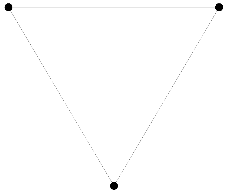
          SAPERE Incarnation

          LSAs

          LSAs, similarly to Prolog terms, support unification and substitution: it is possible to create tuple templates, match them against sets of ground tuples, and obtain a matching ground tuple as result.

          A tuple argument is considered a variable if it begins with an uppercase letter. Additionally, it is possible to discard some matches by expressing constraints on values.

          Ground LSA syntax

          GroundLSA ::= GroundArgument (',' GroundArgument)*
          GroundArgument ::= Number | Atom | Set
          Atom ::= [a-z]([a-z]|[A-Z]|[0-9])*
          Number ::= [0-9]+('.'[0-9]*)
          Set ::= '[' ((Atom | Number)';')* ']'

          LSA Syntax

          LSA ::= '{' GroundLSA | TemplateLSA '}'
          TemplateLSA ::= Argument (',' Argument)*
          Argument ::= GroundArgument | Variable | Constraint
          Variable ::= [A-Z]([a-z]|[A-Z]|[0-9])*
          Constraint ::= 'def:' Variable Operation
          Operation ::= ('>'|'>'|'='|'!=') Number | 'add ' Variable | 'del ' Variable

          Swing GUI

          The current, Swing-based graphical interface for Alchemist is being replaced by a new, JavaFX-based interface. This page currently hosts minimal information on how to use such legacy GUI.

          Shortcuts

          Key binding Active Effect
          L always (En/Dis)ables the painting of links between nodes
          M always (En/Dis)ables the painting of a marker on the closest node
          Mouse pan in normal mode Moves around
          Mouse wheel in normal mode Zooms in/out
          Double click in normal mode Opens a frame with the closest node information
          Right click in normal mode Enters screen rotation mode
          P always Plays/pauses the simulation
          R always Enables the real-time mode
          Left arrow always Speeds the simulation down (more calls to the graphics)
          Right arrow always Speeds the simulation up (less calls to the graphics)
          S always Enters / exits the select mode (nodes can be selected with the mouse)
          O in select mode Selected nodes can be moved by drag and drop
          E in select mode Enters edit mode (to manually change node contents)